About Me

Principal Data Scientist @ Monetate Labs • PyMC3 contributor
@AustinRochford • austinrochford.com • github.com/AustinRochford
austin.rochford@gmail.com • arochford@monetate.com
About this Talk
Last Two Minute Report

Scraping the data
Loading the data
In [12]:
orig_df.head(n=2).T
Out[12]:
Research questions
- How does game context impact foul calls?
- Is (not) committing and/or drawing fouls a measurable player skill?
Exploratory Data Analysis
In [14]:
(orig_df.call_type
        .str.split(':', expand=True).iloc[:, 0]
        .value_counts()
        .plot(kind='bar', color=blue, logy=True, title="Call types")
        .set_ylabel("Frequency"));

In [16]:
(foul_df.call_type
        .str.split(': ', expand=True).iloc[:, 1]
        .value_counts()
        .plot(kind='bar', color=blue, logy=True, title="Foul Types")
        .set_ylabel("Frequency"));

Data transformation
In [25]:
df.head(n=2).T
Out[25]:
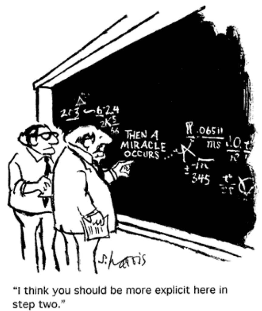
Modeling

|
George Box (via Dustin Tran):
|
Build a model of the science
In [27]:
make_foul_rate_yaxis(
    df.pivot_table('foul_called', 'season')
      .rename(index=season_enc.inverse_transform)
      .rename_axis("Season")
      .plot(kind='bar', rot=0, legend=False)
);

- Each season has a different foul call rate
In [28]:
import pymc3 as pm

with pm.Model() as base_model:
    β_season = pm.Normal('β_season', 0., 5., shape=n_season)
    p = pm.Deterministic('p', pm.math.sigmoid(β_season))
- Foul calls are like flipping a weighted coin
In [30]:
with base_model:
    y = pm.Bernoulli(
        'y', p[season],
        observed=df.foul_called.values
    )
Infer the model given data

|

|
In [32]:
with base_model:
    base_trace = pm.sample(**SAMPLE_KWARGS)
Convergence diagnostics
The folk theorem [of statistical computing] is this: When you have computational problems, often there’s a problem with your model.
In [35]:
(pm.energyplot(base_trace, legend=False, figsize=(6, 4))
   .set_title(CONVERGENCE_TITLE()));

Criticize the model given data
In [38]:
resid_df = (df.assign(p_hat=base_trace['p'][:, df.season].mean(axis=0))
              .assign(resid=lambda df: df.foul_called - df.p_hat))
In [39]:
resid_df[['foul_called', 'p_hat', 'resid']].head()
Out[39]:
In [40]:
(resid_df.pivot_table('resid', 'season')
         .rename(index=season_enc.inverse_transform))
Out[40]:
Intentional fouls
 |
 |
In [42]:
make_time_axes(
    resid_df.pivot_table('resid', 'seconds_left')
            .reset_index()
            .plot('seconds_left', 'resid', kind='scatter'),
    ylabel="Residual"
);

Build a model of the science, take two
In [44]:
make_time_axes(
    df.pivot_table('foul_called', 'seconds_left', 'trailing_committing')
      .rolling(20).mean()
      .rename(columns={0: "No", 1: "Yes"})
      .rename_axis("Committing team is trailing", axis=1)
      .plot()
);

In [45]:
ax = (df.pivot_table('foul_called', 'call_type')
        .rename(index=call_type_enc.inverse_transform)
        .rename_axis("Call type", axis=0)
        .plot(kind='barh', legend=False))
ax.xaxis.set_major_formatter(pct_formatter);
ax.set_xlabel("Observed foul call rate");

- Each call type has a different foul call rate
In [48]:
with poss_model:
    β_call = hierarchical_normal('β_call', n_call_type)
In [51]:
make_time_axes(
    df.pivot_table('foul_called', 'seconds_left', 'trailing_poss')
      .loc[:, 1:3]
      .rolling(20).mean()
      .rename_axis(
          "Trailing possessions\n(committing team)",
          axis=1
      )
      .plot()
);

In [52]:
make_time_axes(
    df.pivot_table('foul_called', 'seconds_left', 'call_type')
      .rolling(20).mean()
      .rename(columns=call_type_enc.inverse_transform)
      .rename_axis(None, axis=1)
      .plot()
);

The shot clock

In [55]:
ax = sns.heatmap(
    df.pivot_table('foul_called', 'trailing_poss', 'remaining_poss')
      .rename_axis(
          "Trailing possessions\n(committing team)", axis=0
      )
      .rename_axis("Remaining possessions", axis=1),
    cmap='seismic', cbar_kws={'format': pct_formatter}
)
ax.invert_yaxis();
ax.set_title("Observed foul call rate");

Difference from call type average
In [58]:
(sns.FacetGrid(diff_df, col='call_type', col_wrap=3, aspect=1.5)
    .map_dataframe(plot_foul_diff_heatmap)
    .set_axis_labels(
        "Remaining possessions",
        "Trailing possessions\n(committing team)"
    )
    .set_titles("{col_name}"));

- The foul call rate changes based on the number of possessions trailing and remaining and the call type
In [59]:
with poss_model:
    β_poss = hierarchical_normal(
        'β_poss',
        (n_trailing_poss, n_remaining_poss, n_call_type),
        σ_shape=(1, 1, n_call_type)
    )
- The foul call rate is a combination of season, call type, and possession factors
In [61]:
with poss_model:
    η_game = β_season[season] \
                + β_call[call_type] \
                + β_poss[
                    trailing_poss, remaining_poss, call_type
                ]
Infer the model given data, take two
In [63]:
with poss_model:
    poss_trace = pm.sample(**SAMPLE_KWARGS)
Criticize the model given data, take two
In [67]:
ax = sns.heatmap(
    resid_df.pivot_table('resid', 'trailing_poss', 'remaining_poss')
      .rename_axis("Trailing possessions\n(committing team)", axis=0)
      .rename_axis("Remaining possessions", axis=1)
      .loc[-3:3],
    cmap='seismic',  cbar_kws={'format': pct_formatter}
)
ax.invert_yaxis();
ax.set_title("Observed foul call rate");

In [69]:
ax = (resid_df.groupby(bins[bin_ix])
              .resid.mean()
              .rename_axis('p_hat', axis=0)
              .reset_index()
              .plot('p_hat', 'resid', kind='scatter'))

ax.xaxis.set_major_formatter(pct_formatter);
ax.set_xlabel(r"Binned $\hat{p}$");

make_foul_rate_yaxis(ax, label="Residual");

In [70]:
ax = (resid_df.groupby('seconds_left')
              .resid.mean()
              .reset_index()
              .plot('seconds_left', 'resid', kind='scatter'))
make_time_axes(ax, ylabel="Residual");

Model selection
In [72]:
comp_df = (pm.compare(
                (base_trace, poss_trace),
                (base_model, poss_model)
             )
             .rename(index=MODEL_NAME_MAP)
             .loc[MODEL_NAME_MAP.values()])
In [73]:
comp_df
Out[73]:
In [74]:
fig, ax = plt.subplots()
ax.errorbar(
    np.arange(len(MODEL_NAME_MAP)), comp_df.WAIC,
    yerr=comp_df.SE, fmt='o'
);
ax.set_xticks(np.arange(len(MODEL_NAME_MAP)));
ax.set_xticklabels(comp_df.index);
ax.set_xlabel("Model");
ax.set_ylabel("WAIC");

Research questions
How does game context impact foul calls?- Is (not) committing and/or drawing fouls a measurable player skill?
Build a model of the science, take three

Item-response theory
In [76]:
fig
Out[76]:

- Each disadvantaged player has an ideal point (per season)
In [79]:
with irt_model:
    θ_player = hierarchical_normal(
        'θ_player', (n_player, n_season)
    )
    θ = θ_player[player_disadvantaged, season]
- Each committing player has an ideal point (per season)
In [80]:
with irt_model:
    b_player = hierarchical_normal(
        'b_player', (n_player, n_season)
    )
    b = b_player[player_committing, season]
- Players affect the foul call rate through the difference in their ideal points
In [81]:
with irt_model:
    η_player = θ - b
- Game and player effects combine to determine the foul call rate
In [82]:
with irt_model:
    η = η_game + η_player
Infer the model given data, take three
In [84]:
with irt_model:
    irt_trace = pm.sample(**SAMPLE_KWARGS)
Criticize the model given data, take three
In [89]:
ax = (resid_df.groupby(bins[bin_ix])
              .resid.mean()
              .rename_axis('p_hat', axis=0)
              .reset_index()
              .plot('p_hat', 'resid', kind='scatter'))
ax.xaxis.set_major_formatter(pct_formatter);
ax.set_xlabel(r"Binned $\hat{p}$");
make_foul_rate_yaxis(ax, label="Residual");

Model selection
In [93]:
fig, ax = plt.subplots()
ax.errorbar(
    np.arange(len(MODEL_NAME_MAP)), comp_df.WAIC,
    yerr=comp_df.SE, fmt='o'
);
ax.set_xticks(np.arange(len(MODEL_NAME_MAP)));
ax.set_xticklabels(comp_df.index);
ax.set_xlabel("Model");
ax.set_ylabel("WAIC");

Is committing and/or drawing fouls a measurable player skill?
In [101]:
fig
Out[101]:

In [104]:
fig, ax = plot_latent_params(
    top_bot_irt_df[top_bot_irt_df.param == 'θ']
                  .sort_values('mean')
)
ax.set_xlabel(r"$\hat{\theta}$");
ax.set_title("Top and bottom ten");

In [105]:
fig, ax = plot_latent_params(
    top_bot_irt_df[top_bot_irt_df.param == 'b']
                  .sort_values('mean')
)
ax.set_xlabel(r"$\hat{b}$");
ax.set_title("Top and bottom ten");

In [106]:
player_irt_df.head()
Out[106]:
Year-over-year consistency (players that appeared in all seasons)
In [110]:
style_grid(sns.PairGrid(player_irt_df.loc[player_all_season], size=1.75)
              .map_upper(plt.scatter, alpha=0.5)
              .map_diag(plt.hist)
              .map_lower(plot_corr));

Year-over-year consistency (players that appeared at least ten times in all seasons)
In [113]:
grid.fig
Out[113]:

Research questions
How does game context impact foul calls?Is (not) committing and/or drawing fouls a measurable player skill?
Visualize the Predictions
In [116]:
import dash
import dash_html_components as html
In [129]:
app = dash.Dash()

app.layout = html.Div(children=[
    html.H1(
        "Understanding NBA Foul Calls with Python"
    ),
    html.Center(TABLE)
])
In [130]:
@app.callback(
    dash.dependencies.Output(
        'irt-param-scatter', 'figure'
    ),
    [
        dash.dependencies.Input(
            'season-dropdown','value'
        ),
        dash.dependencies.Input(
            'player-committing-dropdown','value'
        ),
        dash.dependencies.Input(
            'player-disadvantaged-dropdown','value'
        )
    ]
)
def update_irt_scatter(season_,
                       player_committing_,
                       player_disadvantaged_):
    irt_df = get_irt_df(
        player_committing_=player_committing_,
        player_disadvantaged_=player_disadvantaged_,
        season_=season_,
    )

    return get_irt_scatter(irt_df)