Introduction to Probabilistic Programming
DataPhilly
July 13, 2016
@Austin Rochford (arochford@monetate.com)
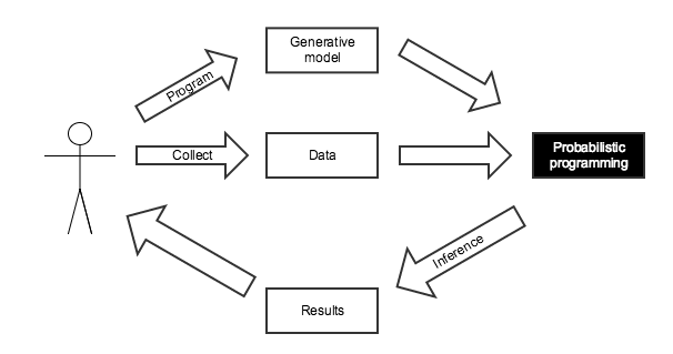
Probabilistic Programming
- Programming with random variables
- User specifies a generative model for the observed data
- "Tell the story" of how the data were created
- The language runtime/software library automatically performs inference
What do we mean by inference?
- Maximum likelihood inference
- Maxumum a posteriori inference
- Full posterior inference

Disease Testing
A certain rare disease affects one in 10,000 people. A test for the disease gives the correct result 99.9% of the time.
What is the probability that a given test is positive?
import pymc3 as pm

with pm.Model() as pretest_disease_model:
    # This is our prior belief about whether or not the subject has the disease,
    # given its prevalence of the disease in the general population
    has_disease = pm.Bernoulli('has_disease', 1e-4)

    # This is the probability of a positive test given the presence or lack
    # of the disease
    p_positive = pm.Deterministic('p_positive',
                                  T.switch(T.eq(has_disease, 1),
                                           # If the subject has the disease,
                                           # this is the probability that the
                                           # test is positive
                                           0.999,
                                           # If the subject does not have the
                                           # disease, this is the probability
                                           # that the test is negative
                                           1 - 0.999))

    # This is the observed test result
    test_positive = pm.Bernoulli('test_positive', p_positive)
samples = 40000
with pretest_disease_model:
    step = pm.Metropolis()
    pretest_disease_trace = pm.sample(samples, step, random_seed=SEED)
pretest_disease_trace['test_positive']
pretest_disease_trace['test_positive'].size
The probability that a given test is positive is
pretest_disease_trace['test_positive'].mean()
0.999 * 1e-4 + (1 - 0.999) * (1 - 1e-4)
If a subject tests positive, what is the probability they have the disease?
with pm.Model() as disease_model:
    # This is our prior belief about whether or not the subject has the disease,
    # given its prevalence of the disease in the general population
    has_disease = pm.Bernoulli('has_disease', 1e-4)

    # This is the probability of a positive test given the presence or lack
    # of the disease
    p_positive = pm.Deterministic('p_positive',
                                  T.switch(T.eq(has_disease, 1),
                                           # If the subject has the disease,
                                           # this is the probability that the
                                           # test is positive
                                           0.999,
                                           # If the subject does not have the
                                           # disease, this is the probability
                                           # that the test is negative
                                           1 - 0.999))

    # This is the observed positive test
    test_positive = pm.Bernoulli('test_positive', p_positive, observed=1)
with disease_model:
    step = pm.Metropolis()
    disease_trace = pm.sample(samples, step, random_seed=SEED)
The probability that someone who tests positive for the disease has it is
disease_trace['has_disease'].mean()
0.999 * 1e-4 / (0.999 * 1e-4 + (1 - 0.999) * (1 - 1e-4))
The Monty Hall Problem

If we select the first door and Monty opens the third to reveal a goat, should we change doors?
with pm.Model() as monty_model:
    # We have no idea where the prize is at the beginning
    prize = pm.DiscreteUniform('prize', 0, 2)

    # The probability that Monty opens each door
    p_open = pm.Deterministic('p_open',
                              T.switch(T.eq(prize, 0),
                                       # If the prize is behind the first door,
                                       # he chooses to open one of the others
                                       # at random
                                       np.array([0., 0.5, 0.5]),
                                       T.switch(T.eq(prize, 1),
                                                # If it is behind the second door,
                                                # he must open the third door
                                                np.array([0., 0., 1.]),
                                                # If it is behind the third door,
                                                # he must open the second door
                                                np.array([0., 1., 0.]))))

    # Monty opened the third door, revealing a goat
    opened = pm.Categorical('opened', p_open, observed=2)
samples = 10000
with monty_model:
    step = pm.Metropolis()
    monty_trace = pm.sample(samples, step, random_seed=SEED)

monty_trace_df = pm.trace_to_dataframe(monty_trace)
monty_trace_df.head()
(monty_trace_df.groupby('prize')
               .size()
               .div(monty_trace_df.shape[0]))
Built on top of theano
- Dynamic generation of
Ccode for models - Automatic differentiation allows for gradient-based inference
- Implements advanced Markov chain Monte carlo algorithms, such at the No U-Turn Sampler
- Implements automatic differentiation variational inference
- Interoperable with both
pandasandpatsy - Provides clean support for multilevel models

A/B Testing

Suppose variant A sees 510 visitors and 40 purchases, but variant B sees 505 visitors and 50 conversions.
with pm.Model() as ab_model:
    # A priori, we have no idea what the purchase rate for variant A will be
    a_rate = pm.Uniform('a_rate')
    # We observed 40 purchases from 510 visitors who saw variant A
    a_purchases = pm.Binomial('a_purchases', 510, a_rate, observed=40)

    # A priori, we have no idea what the purchase rate for variant B will be
    b_rate = pm.Uniform('b_rate')
    # We observed 40 purchases from 510 visitors who saw variant A
    b_purchases = pm.Binomial('b_purchases', 505, b_rate, observed=45)
samples = 10000
with ab_model:
    step = pm.NUTS()
    ab_trace = pm.sample(samples, step, random_seed=SEED)
fig

The probability that variant B is better than variant A is
(ab_trace['a_rate'] < ab_trace['b_rate']).mean()
Robust Regression
fig

fig

with pm.Model() as ols_model:
    # alpha is the slope and beta is the intercept
    alpha = pm.Uniform('alpha', -100, 100)
    beta = pm.Uniform('beta', -100, 100)

    # Ordinary least squares assumes that the noise is normally distributed
    y_obs = pm.Normal('y_obs', alpha + beta * x, 1., observed=y)
samples = 10000
with ols_model:
    step = pm.Metropolis()
    ols_trace = pm.sample(samples, step, random_seed=SEED)
post_y = ols_trace['alpha'] + np.outer(plot_X[:, 1], ols_trace['beta'])
fig

fig

with pm.Model() as robust_model:
    # alpha is the slope and beta is the intercept
    alpha = pm.Uniform('alpha', -100, 100)
    beta = pm.Uniform('beta', -100, 100)

    # t-distributed residuals are less sensitive to outliers
    y_obs = pm.StudentT('y_obs', nu=3., mu=alpha + beta * x, observed=y)
with robust_model:
    step = pm.Metropolis()

    robust_trace = pm.sample(samples, step, random_seed=SEED)
post_y_robust = robust_trace['alpha'] + np.outer(plot_X[:, 1], robust_trace['beta'])
fig

Congressional Ideal Point Model
df.head()
parties
grid.fig

$p_{i, j}$ is the probability that representative $i$ votes for bill $j$.
$$ \begin{align*} \log \left(\frac{p_{i, j}}{1 - p_{i, j}}\right) & = \gamma_j \left(\alpha_i - \beta_j\right) \\ & = \textrm{ability of bill } j \textrm{ to discriminate} \times (\textrm{conservativity of represetative } i\ - \textrm{conservativity of bill } j) \end{align*} $$with pm.Model() as ideal_point_model:
# The conservativity of representative i
alpha = pm.Normal('alpha', 0, 1., shape=N_REPS)
# The conservativity of bill j
mu_beta = pm.Normal('mu_beta', 0, 1e-3)
sigma_beta = pm.Uniform('sigma_beta', 0, 1e2)
beta = pm.Normal('beta', mu_beta, sd=sigma_beta, shape=N_BILLS)
# The ability of bill j to discriminate
mu_gamma = pm.Normal('mu_gamma', 0, 1e-3)
sigma_gamma = pm.Uniform('sigma_gamma', 0, 1e2)
gamma = pm.Normal('gamma', mu_gamma, sd=sigma_gamma, shape=N_BILLS)
# The probability that representative i votes for bill j
p = pm.Deterministic('p', T.nnet.sigmoid(gamma[vote_df.bill] * (alpha[vote_df.rep] - beta[vote_df.bill])))
# The observed votes
vote = pm.Bernoulli('vote', p, observed=vote_df.vote)
samples = 20000
with ideal_point_model:
    step = pm.Metropolis()
    ideal_point_trace = pm.sample(samples, step, random_seed=SEED)
rep_alpha = ideal_point_trace['alpha'].mean(axis=0)
fig

pm.forestplot(ideal_point_trace, varnames=['gamma']);


Source: http://mqscores.berkeley.edu/


References

Probabilistic Programming and Bayesian Methods for Hackers (Open source, uses PyMC2, PyMC3 port in progress)
Think Bayes (Available freely online, calculations in Python)