Open Source Bayesian Inference in Python with PyMC3
FOSSCON • Philadelphia • August 26, 2017
@AustinRochford
Who am I?

@AustinRochford • GitHub • Website
austin.rochford@gmail.com • arochford@monetate.com
PyMC3 developer • Principal Data Scientist at Monetate Labs
Bayesian Inference
A motivating question:
A rare disease is present in one out of one hundred thousand people. A test gives the correct diagnosis 99.9% of the time. What is the probability that a person that tests positive has the disease?
Conditional Probability
Conditional probability is the probability that one event will happen, given that another event has occured.
Our question,
A rare disease is present in one out of one hundred thousand people. A test gives the correct diagnosis 99.9% of the time. What is the probability that a person that tests positive has the disease?
becomes

0.999 * 1e-5 / (0.999 * 1e-5 + 0.001 * (1 - 1e-5))
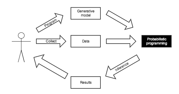
Probabilistic Programming for Bayesian Inference

We know the disease is present in one in one hundred thousand people.
import pymc3 as pm

with pm.Model() as disease_model:
    has_disease = pm.Bernoulli('has_disease', 1e-5)
If a person has the disease, there is a 99.9% chance they test positive. If they do not have the disease, there is a 0.1% chance they test positive.
with disease_model:
    p_test_pos = has_disease * 0.999 + (1 - has_disease) * 0.001
This person has tested positive for the disease.
with disease_model:
    test_pos = pm.Bernoulli('test_pos', p_test_pos, observed=1)
What is the probability that this person has the disease?
with disease_model:
    disease_trace = pm.sample(draws=10000, random_seed=SEED)
disease_trace['has_disease']
disease_trace['has_disease'].mean()
0.999 * 1e-5 / (0.999 * 1e-5 + 0.001 * (1 - 1e-5))
Monte Carlo Methods
N = 5000

x, y = np.random.uniform(0, 1, size=(2, N))
fig

in_circle = x**2 + y**2 <= 1
fig

4 * in_circle.mean()
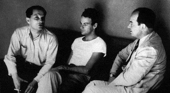
History of Monte Carlo Methods
The Monty Hall Problem

Initially, we have no information about which door the prize is behind.
with pm.Model() as monty_model:
    prize = pm.DiscreteUniform('prize', 0, 2)
If we choose door one:
| Prize behind | Door 1 | Door 2 | Door 3 |
|---|---|---|---|
| Door 1 | No | Yes | Yes |
| Door 2 | No | No | Yes |
| Door 2 | No | Yes | No |
from theano import tensor as tt

with monty_model:
    p_open = pm.Deterministic('p_open',
                              tt.switch(tt.eq(prize, 0),
                                        # it is behind the first door
                                        np.array([0., 0.5, 0.5]),
                              tt.switch(tt.eq(prize, 1),
                                        # it is behind the second door
                                        np.array([0., 0., 1.]),
                                        # it is behind the third door
                                        np.array([0., 1., 0.]))))
Monty opened the third door, revealing a goat.
with monty_model:
    opened = pm.Categorical('opened', p_open, observed=2)
Should we switch our choice of door?
with monty_model:
    monty_trace = pm.sample(draws=10000, random_seed=SEED)

monty_df = pm.trace_to_dataframe(monty_trace)
monty_df.prize.head()
fig

Yes, we should switch our choice of door.
Introduction to PyMC3
From the PyMC3 documentation:
PyMC3 is a Python package for Bayesian statistical modeling and Probabilistic Machine Learning which focuses on advanced Markov chain Monte Carlo and variational fitting algorithms. Its flexibility and extensibility make it applicable to a large suite of problems.
![]()

As of October 2016, PyMC3 is a NumFOCUS fiscally sponsored project.
Features
- Uses Theano as a computational backend
- Automated differentiation, dynamic C compilation, GPU integration
- Implements Hamiltonian Monte Carlo and No-U-Turn sampling
- High-level GLM (
R-like syntax) and Gaussian process specification - General framework for variational inference


Case Study: Sleep Deprivation

sleep_df.head()
fig

Each subject has a baseline reaction time, which should not be too far apart.
with pm.Model() as sleep_model:
    μ_α = pm.Normal('μ_α', 0., 5.)
    σ_α = pm.HalfCauchy('σ_α', 5.)
    α = pm.Normal('α', μ_α, σ_α, shape=n_subjects)
Each subject's reaction time increases at a different rate after days of sleep deprivation.
with sleep_model:
    μ_β = pm.Normal('μ_β', 0., 5.)
    σ_β = pm.HalfCauchy('σ_β', 5.)
    β = pm.Normal('β', μ_β, σ_β, shape=n_subjects)
The baseline reaction time and rate of increase lead to the observed reaction times.
with sleep_model:
    μ = pm.Deterministic('μ', α[subject_ix] + β[subject_ix] * days)
    σ = pm.HalfCauchy('σ', 5.)
    obs = pm.Normal('obs', μ, σ, observed=reaction_std)
N_JOBS = 3
JOB_SEEDS = [SEED + i for i in range(N_JOBS)]

with sleep_model:
    sleep_trace = pm.sample(njobs=N_JOBS, random_seed=JOB_SEEDS)
Convergence Diagnostics
ax = pm.energyplot(sleep_trace, legend=False)
ax.set_title("BFMI = {:.3f}".format(pm.bfmi(sleep_trace)));

max(np.max(gr_values) for gr_values in pm.gelman_rubin(sleep_trace).values())
Prediction
with sleep_model:
    pp_sleep_trace = pm.sample_ppc(sleep_trace)
pp_df.head()
grid.fig

Hamiltonian Monte Carlo in PyMC3
mcmc_fig

The Curse of Dimensionality
fig

Hamiltonian Monte Carlo

x = tt.dscalar('x')
x.tag.test_value = 0.

y = x**3
from theano import pprint

pprint(tt.grad(y, x))
Case Study: 1984 Congressional Votes
vote_df.head()
Question: can we separate Democrats and Republicans based on their voting records?
grid.fig

Latent State Model
- Representatives ($\color{blue}{\theta_i}$) and bills ($\color{green}{b_j})$ have ideal points on a liberal-conservative spectrum.
- If the ideal points are equal, there is a 50% chance the representative will vote for the bill.
with pm.Model() as vote_model:
    # representative ideal points
    θ = pm.Normal('θ', 0., 1., shape=n_rep)

    # bill ideal points
    a = hierarchical_normal('a', N_BILL)
- Bills also have an ability to discriminate ($\color{red}{a_j}$) between conservative and liberal representatives.
- Some bills have broad bipartisan support, while some provoke votes along party lines.
with vote_model:
    # bill discrimination parameters
    b = hierarchical_normal('b', N_BILL)
This model has
n_rep + 2 * (N_BILL + 1)
parameters
Observation Model
$$ \begin{align*} P(\textrm{Representative }i \textrm{ votes for bill }j\ |\ \color{blue}{\theta_i}, \color{green}{b_j}, \color{red}{a_j}) & = \frac{1}{1 + \exp\left(-\left(\color{red}{a_j} \cdot \color{blue}{\theta_i} - \color{green}{b_j}\right)\right)} \end{align*} $$fig

with vote_model:
    η = a[bill_id] * θ[rep_id] - b[bill_id]
    p = pm.math.sigmoid(η)

    obs = pm.Bernoulli('obs', p, observed=vote)
Hamiltonian Monte Carlo Inference
with vote_model:
    nuts_trace = pm.sample(init='adapt_diag', njobs=N_JOBS,
                           random_seed=JOB_SEEDS)
Convergence Diagnostics
ax = pm.energyplot(nuts_trace, legend=False)
ax.set_title("BFMI = {:.3f}".format(pm.bfmi(nuts_trace)));

max(np.max(gr_values) for gr_values in pm.gelman_rubin(nuts_trace).values())
Ideal Points
fig

Discriminative Ability of Bills
pm.forestplot(nuts_trace, varnames=['a'], rhat=False, xtitle="$a$",
              ylabels=["Bill {}".format(i + 1) for i in range(N_BILL)]);

Comparison to Non-Hamiltonian MCMC
with vote_model:
    step = pm.Metropolis()
    met_trace_ = pm.sample(10000, step, njobs=N_JOBS, random_seed=JOB_SEEDS)

met_trace = met_trace_[5000::5]
max(np.max(gr_values) for gr_values in pm.gelman_rubin(met_trace).values())
fig

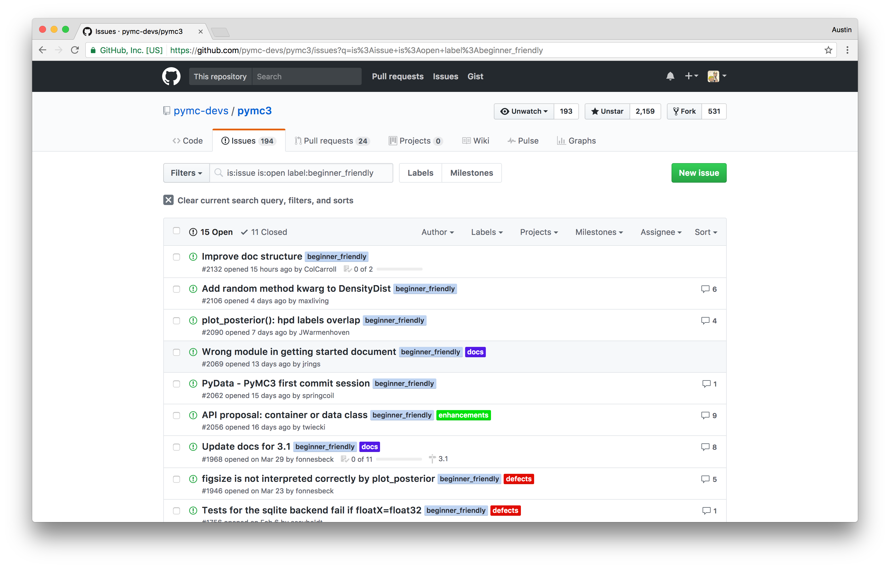
Next Steps
PyMC3
|
|

|

|
Probabilistic Programming Ecosystem
| Probabilistic Programming System | Language | License | Discrete Variable Support | Automatic Differentiation/Hamiltonian Monte Carlo | Variational Inference |
|---|---|---|---|---|---|
| PyMC3 | Python | Apache V2 | Yes | Yes | Yes |
| Stan | C++, R, Python, ... | BSD 3-clause | No | Yes | Yes |
| Edward | Python, ... | Apache V2 | Yes | Yes | Yes |
| BUGS | Standalone program, R | GPL V2 | Yes | No | No |
| JAGS | Standalone program, R | GPL V2 | Yes | No | No |
Thank you!

@AustinRochford • austin.rochford@gmail.com • arochford@monetate.com
The Jupyter notebook used to generate these slides is available here.