About Me

@AustinRochford • austinrochford.com • github.com/AustinRochford
austin.rochford@gmail.com • arochford@monetate.com
PyMC3 contributor • Principal Data Scientist at Monetate Labs
Probabilistic Programming
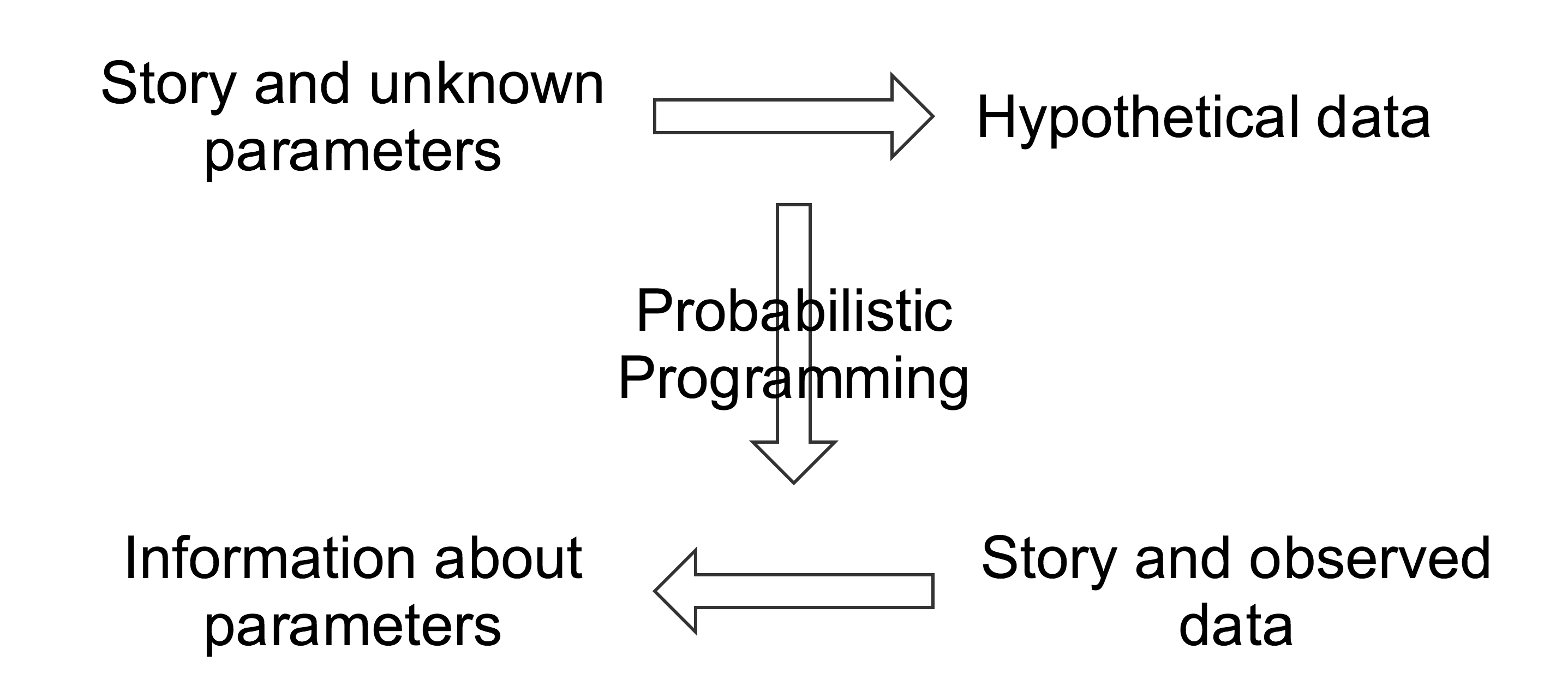
- Write a program to simulate the data generating process
- Language runtime/software library performs inference
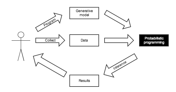
Data Science — inference enables storytelling
Probabilistic Programming — storytelling enables inference
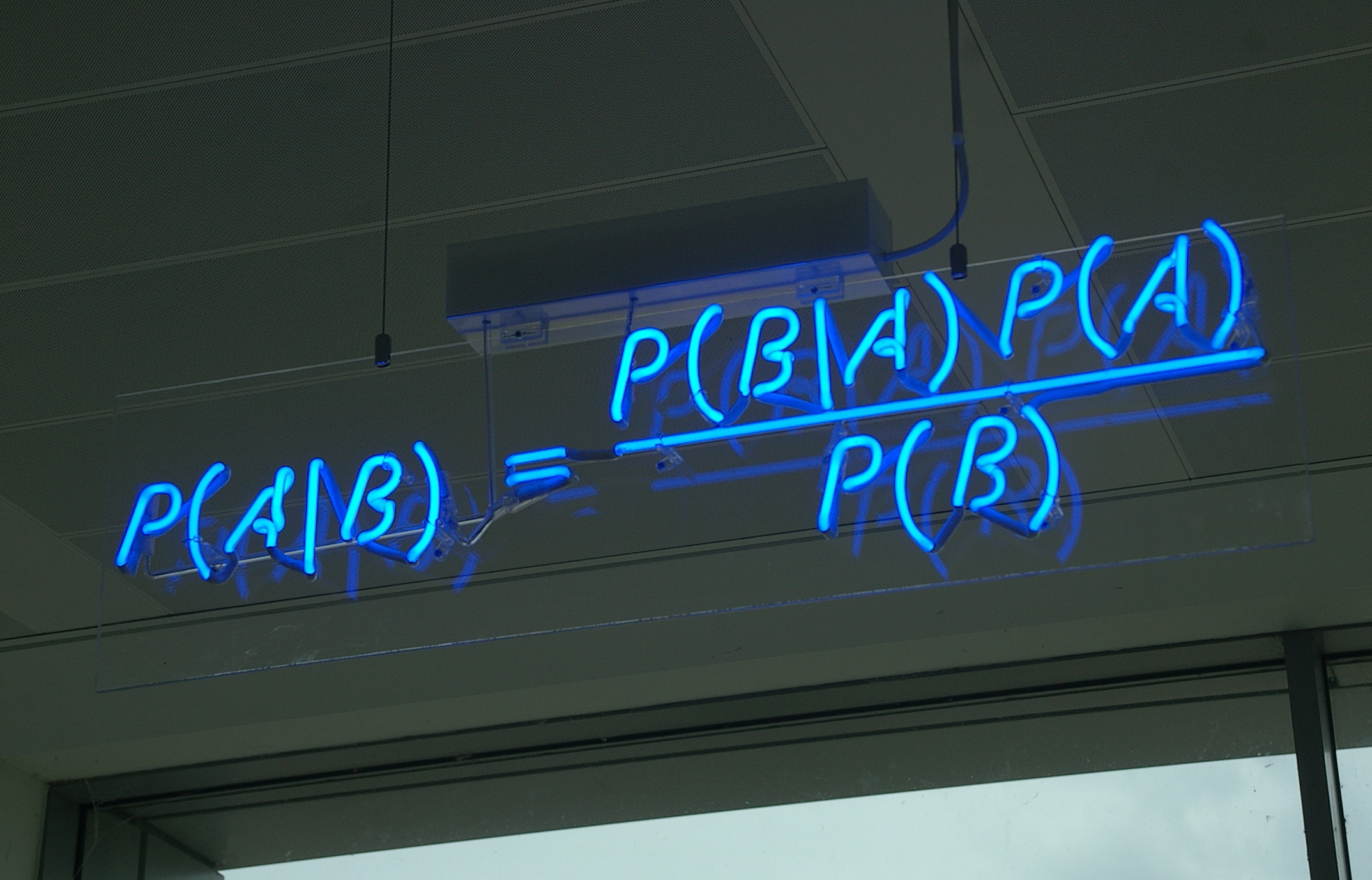
Enter: Bayes theorem
Benefits of probabilistic programming
- Model-agnostic inference algorithms
- Quantification of uncertainty
- Incorporation of domain knowledge
- Modularity
Initially, we have no information about which door the prize is behind.
import pymc3 as pm

with pm.Model() as monty_model:
    prize = pm.DiscreteUniform('prize', 0, 2)
If we choose door one:
| Prize behind | Door 1 | Door 2 | Door 3 |
|---|---|---|---|
| Door 1 | No | Yes | Yes |
| Door 2 | No | No | Yes |
| Door 2 | No | Yes | No |
from theano import tensor as tt

with monty_model:
    p_open = pm.Deterministic('p_open',
                              tt.switch(tt.eq(prize, 0),
                                        # it is behind the first door
                                        np.array([0., 0.5, 0.5]),
                              tt.switch(tt.eq(prize, 1),
                                        # it is behind the second door
                                        np.array([0., 0., 1.]),
                                        # it is behind the third door
                                        np.array([0., 1., 0.]))))
Monty opened the third door, revealing a goat.

with monty_model:
    opened = pm.Categorical('opened', p_open, observed=2)
Should we switch our choice of door?
with monty_model:
    monty_trace = pm.sample(1000, init=None, random_seed=SEED)

monty_df = pm.trace_to_dataframe(monty_trace)
monty_df.head()
monty_df.prize.mean()
fig

From the PyMC3 documentation:
PyMC3 is a Python package for Bayesian statistical modeling and Probabilistic Machine Learning which focuses on advanced Markov chain Monte Carlo and variational fitting algorithms. Its flexibility and extensibility make it applicable to a large suite of problems.
![]()
PyMC3 features
- Uses Theano as a computational backend
- Automated differentiation, dynamic C compilation, GPU integration
- Implements Hamiltonian Monte Carlo and No-U-Turn sampling
- High-level GLM (
R-like syntax) and Gaussian process specification - Provides a framework for operator variational inference
HTML(mcmc_video)
Statistical workflow
- Tell a story about how the data may have been generated
- Encode that story as a probabilistic model
- Perform inference
- Check model diagnostics
- Compare models
- Iterate (
GOTO 1)
Statistical LEGOs

Case study: NBA foul calls

Last two minute report
nba_df.head()
Story
Close basketball games usually end with intentional fouls.
fig

Model
The foul call probability varies over time.
seconds_left_ = theano.shared(seconds_left)

with pm.Model() as nba_model:
    β = pm.GaussianRandomWalk('β', tau=PRIOR_PREC, init=pm.Normal.dist(0., 10.),
                              shape=n_sec)
Transform logodds to probabilities, specify observation model.
with nba_model:
    p = pm.math.sigmoid(β[seconds_left_])
    fc = pm.Bernoulli('fc', p, observed=foul_called)
Inference
nba_trace = sample_from_model(nba_model)
- Automatic sampler assignment (manually configurable)
- Automatic initialization of HMC/NUTS using ADVI
Model diagnostics — posterior predictions
To sample from the posterior predictive distribution, we change the value of the Theano shared variable seconds_left_.
pp_sec = np.arange(n_sec)
seconds_left_.set_value(pp_sec)

with nba_model:
    pp_nba_trace = pm.sample_ppc(nba_trace, N_PP_SAMPLES)
fig

Model diagnostics — sampling
The folk theorem [of statistical computing] is this: When you have computational problems, often there’s a problem with your model.
pm.energyplot(nba_trace).legend(bbox_to_anchor=(0.6, 1));

Model selection
PyMC3 can calculate:
- Deviance information criterion (DIC)
- Bayesian predictive information criterion (BPIC)
- Widely applicable/Watanabe-Akaike information criterion (WAIC)
with nba_model:
    nba_waic = pm.waic(nba_trace)

print(nba_waic)
Story — take two
The trailing team has more incentive to foul than the leading team.
fig

Model and inference
There is a base rate at which fouls are called.
with pm.Model() as trailing_model:
    α = pm.Normal('α', 0., 10.)
The trailing team is more likely to commit fouls as the game nears its end.
seconds_left_.set_value(seconds_left)
committing_trailing_ = theano.shared(1. * (score_diff < 0))

with trailing_model:
    β = pm.GaussianRandomWalk('β', tau=PRIOR_PREC, init=pm.Normal.dist(0., 10.),
                              shape=n_sec)
    η = α + committing_trailing_ * β[seconds_left_]
trailing_trace = sample_from_model(trailing_model, quiet=True)
Model diagnostics — posterior prediction
fig

Model selection
fig

Story — take three
Larger score differences incentivize the trailing team to foul sooner and more aggressively.
fig

Model and inference
There is a base rate at which fouls are called, and the trailing team is more likely to commit fouls as the game nears its end.
seconds_left_.set_value(seconds_left)
committing_trailing_ = theano.shared(1. * (score_diff < 0))

with pm.Model() as diff_model:
    α = pm.Normal('α', 0., 10.)
    β = pm.GaussianRandomWalk('β', tau=PRIOR_PREC, init=pm.Normal.dist(0., 10.),
                              shape=n_sec)
The teams trailing by more points foul more agressively and sooner.
score_diff_ = theano.shared(score_diff)

with diff_model:
    γ = pm.Normal('γ', 0., 10.)
    θ = pm.Normal('θ', 0., 10.)
    λ = pm.math.sigmoid(γ + θ * score_diff_)

    η = α + committing_trailing_ * λ * β[seconds_left_]
diff_trace = sample_from_model(diff_model, quiet=True)
fig

Model selection
fig

Getting started with PyMC3
|
|

|

|

Probabilistic Programming Ecosystem
| Probabilistic Programming System | Language | Discrete Variable Support | Automatic Differentiation/Hamiltonian Monte Carlo | Variational Inference |
|---|---|---|---|---|
| PyMC3 | Python | Yes | Yes | Yes |
| Stan | C++, R, Python, ... | No | Yes | Yes |
| Edward | Python, ... | Yes | Yes | Yes |
| BUGS | Standalone program, R | Yes | No | No |
| JAGS | Standalone program, R | Yes | No | No |