In [11]:
orig_df.head(n=2).T
Out[11]:
| play_id | 20150301CLEHOU-0 | 20150301CLEHOU-1 |
|---|---|---|
| period | Q4 | Q4 |
| seconds_left | 112 | 103 |
| call_type | Foul: Shooting | Foul: Shooting |
| committing_player | Josh Smith | J.R. Smith |
| disadvantaged_player | Kevin Love | James Harden |
| review_decision | CNC | CC |
| away | CLE | CLE |
| home | HOU | HOU |
| date | 2015-03-01 00:00:00 | 2015-03-01 00:00:00 |
| score_away | 103 | 103 |
| score_home | 105 | 105 |
| disadvantaged_team | CLE | HOU |
| committing_team | HOU | CLE |
In [19]:
df.head()
Out[19]:
| seconds_left | foul_called | player_committing | player_disadvantaged | score_committing | score_disadvantaged | season | |
|---|---|---|---|---|---|---|---|
| play_id | |||||||
| 20151028INDTOR-1 | 89.0 | 1.0 | 162 | 98 | 99.0 | 106.0 | 0 |
| 20151028INDTOR-2 | 73.0 | 0.0 | 36 | 358 | 106.0 | 99.0 | 0 |
| 20151028INDTOR-3 | 38.0 | 1.0 | 229 | 222 | 99.0 | 106.0 | 0 |
| 20151028INDTOR-4 | 30.0 | 0.0 | 229 | 98 | 99.0 | 106.0 | 0 |
| 20151028INDTOR-6 | 24.0 | 0.0 | 229 | 100 | 99.0 | 106.0 | 0 |
Model outline
$$ \operatorname{log-odds}(\textrm{Foul}) \ \sim \textrm{Season factor} + \left(\textrm{Disadvantaged skill} - \textrm{Committing skill}\right) $$
In [22]:
with pm.Model() as irt_model:
    β_season = pm.Normal('β_season', 0., 2.5, shape=n_season)

    θ = hierarchical_normal('θ', n_player) # disadvantaged skill
    b = hierarchical_normal('b', n_player) # committing skill

    p = pm.math.sigmoid(
        β_season[season] + θ[player_disadvantaged] - b[player_committing]
    )

    obs = pm.Bernoulli(
        'obs', p,
        observed=df['foul_called'].values
    )
In [24]:
with irt_model:
    trace = pm.sample(500, **SAMPLE_KWARGS)
Auto-assigning NUTS sampler...
Initializing NUTS using jitter+adapt_diag...
Multiprocess sampling (3 chains in 3 jobs)
NUTS: [σ_b, Δ_b, σ_θ, Δ_θ, β_season]
Sampling 3 chains: 100%|██████████| 3000/3000 [02:07<00:00, 23.58draws/s]
In [26]:
az.rhat(trace).max()
Out[26]:
<xarray.Dataset>
Dimensions:   ()
Data variables:
    β_season  float64 1.0
    Δ_θ       float64 1.01
    Δ_b       float64 1.0
    σ_θ       float64 1.01
    θ         float64 1.01
    σ_b       float64 1.0
    b         float64 1.0
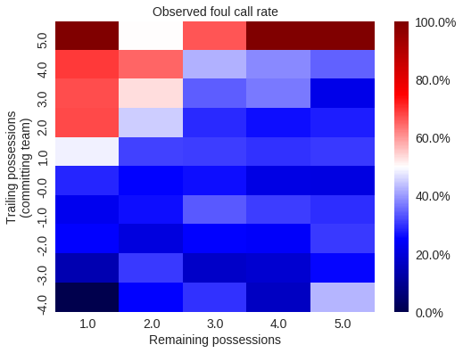
Basketball strategy leads to more complexity

In [31]:
fig
Out[31]:
The shot clock

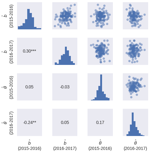
Are we measuring a skill?
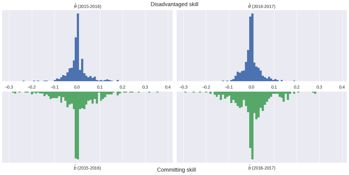
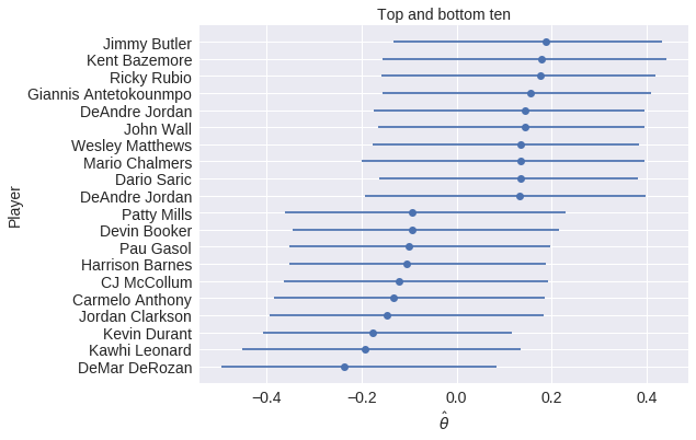
|
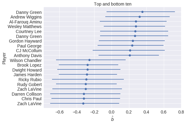
|
Future Work
- Advanced baseball stats
- Hockey
- Faceoff skills
- Fighting ability

