Capture-Recapture Models in Python with PyMC3
Recently, a project at work has led me to learn a bit about capture-recapture models for estimating the size and dynamics of populations that cannot be fully enumerated. These models often arise in ecological statistics when estimating the size, birth, and survival rates of animal populations in the wild. This post gives examples of implementing three capture-recapture models in Python with PyMC3 and is intended primarily as a reference for my future self, though I hope it may serve as a useful introduction for others as well.
We will implement three Bayesian capture-recapture models:
- the Lincoln-Petersen model of abundance,
- the Cormack-Jolly-Seber model of survival, and
- the Jolly-Seber model of abundance and survival.
%matplotlib inlineimport loggingfrom matplotlib import pyplot as plt
from matplotlib.ticker import StrMethodFormatter
import numpy as np
import pymc3 as pm
from pymc3.distributions.dist_math import binomln, bound, factln
import scipy as sp
import seaborn as sns
import theano
from theano import tensor as ttsns.set()
PCT_FORMATTER = StrMethodFormatter('{x:.1%}')SEED = 518302 # from random.org, for reproducibility
np.random.seed(SEED)# keep theano from complaining about compile locks
(logging.getLogger('theano.gof.compilelock')
.setLevel(logging.CRITICAL))
# keep theano from warning about default rounding mode changes
theano.config.warn.round = FalseThe Lincoln-Petersen model
The simplest model of abundace, that is, the size of a population, is the Lincoln-Petersen model. While this model is a bit simple for most practical applications, it will introduce some useful modeling concepts and computational techniques.
The idea of the Lincoln-Petersen model is to visit the observation site twice to capture individuals from the population of interest. The individuals captured during the first visit are marked (often with tags, radio collars, microchips, etc.) and then released. The number of individuals captured, marked, and released is recorded as \(n_1\). On the second visit, the number of captured individuals is recorded as \(n_2\). If enough individuals are captured on the second visit, chances are quite high that several of them will have been marked on the first visit. The number of marked individuals recaptured on the second visit is recorded as \(n_{1, 2}\).
The Lincoln-Petersen model assumes that: 1. each individuals has an equal probability to be captured on both visits (regardless of whether or not they were marked), 2. no marks fall off or become illegible, and 3. the population is closed, that is, no individuals are born, die, enter, or leave the site between visits.
The third assumption is quite restrictive, and will be relaxed in the two subsequent models. The first two assumptions can be relaxed in various ways, but we will not do so in this post. First we derive a simple analytic estimator for the total population size given \(n_1\), \(n_2\), and \(n_{1, 2}\), then we fit a Bayesian Lincoln-Petersen model using PyMC3 to set the stage for the (Cormack-)Jolly-Seber models.
Let \(N\) denote the size of the unknown total population, and let \(p\) denote the capture probability. We have that
\[ \begin{align*} n_1, n_2\ |\ N, p & \sim \textrm{Bin}(N, p) \\ n_{1, 2}\ |\ n_1, p & \sim \textrm{Bin}(n_1, p). \end{align*} \]
Therefore \(\frac{n_2}{N}\) and \(\frac{n_{1, 2}}{n_1}\) are unbiased estimates of \(p\). The Lincoln-Peterson estimator is derived by equating these estimators
\[\frac{n_2}{\hat{N}} = \frac{n_{1, 2}}{n_1}\]
and solving for
\[\hat{N} = \frac{n_1 n_2}{n_{1, 2}}.\]
We now simulate a data set where \(N = 1000\) and the capture probability is \(p = 0.1\)
N_LP = 1000
P_LP = 0.1

x_lp = sp.stats.bernoulli.rvs(P_LP, size=(2, N_LP))
The rows of x_lp correspond to site visits and the columns to individuals. The entry x_lp[i, j] is one if the \(j\)-th individuals was captured on the \(i\)-th site visit, and zero otherwise.
x_lparray([[0, 0, 0, ..., 0, 0, 0],
[0, 0, 0, ..., 0, 1, 0]])We construct \(n_1\), \(n_2\), and \(n_{1, 2}\) from x_lp.
n1, n2 = x_lp.sum(axis=1)
n12 = x_lp.prod(axis=0).sum()
n1, n2, n12(109, 95, 10)The Lincoln-Petersen estimate of \(N\) is therefore
N_lp = n1 * n2 / n12

N_lp1035.5We now give a Bayesian formulation of the Lincoln-Petersen model. We use the priors
\[ \begin{align*} p & \sim U(0, 1) \\ \pi(N) & = 1 \textrm{ for } N \geq n_1 + n_2 - n_{1, 2}. \end{align*} \]
Note that the prior on \(N\) is improper.
with pm.Model() as lp_model:
    p = pm.Uniform('p', 0., 1.)
    N_ = pm.Bound(pm.Flat, lower=n1 + n2 - n12)('N')
We now implement the likelihoods of the data given above during the derivation of the Lincoln-Petersen estimator.
with lp_model:
    n1_obs = pm.Binomial('n1_obs', N_, p, observed=n1)
    n2_obs = pm.Binomial('n2_obs', N_, p, observed=n2)
    n12_obs = pm.Binomial('n12_obs', n1, p, observed=n12)
Now that the model is fully specified, we sample from its posterior distribution.
NJOBS = 3

SAMPLE_KWARGS = {
    'draws': 1000,
    'njobs': NJOBS,
    'random_seed': [SEED + i for i in range(NJOBS)],
    'nuts_kwargs': {'target_accept': 0.9}
}
with lp_model:
lp_trace = pm.sample(**SAMPLE_KWARGS)Auto-assigning NUTS sampler...
Initializing NUTS using jitter+adapt_diag...
Multiprocess sampling (3 chains in 3 jobs)
NUTS: [N_lowerbound__, p_interval__]
100%|██████████| 1500/1500 [00:06<00:00, 230.30it/s]
The number of effective samples is smaller than 25% for some parameters.First we examine a few sampling diagnostics. The Bayesian fraction of missing information (BFMI) and energy plot give no cause for concern.
pm.bfmi(lp_trace)1.0584389661341544pm.energyplot(lp_trace);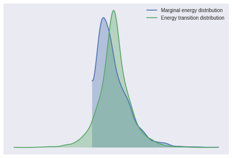
The Gelman-Rubin statistics are close to one, indicating convergence.
max(np.max(gr_stats) for gr_stats in pm.gelman_rubin(lp_trace).values())1.0040982739011743Since there are no apparent sampling problems, we examine the estimate of the population size.
pm.plot_posterior(
    lp_trace, varnames=['N'],
    ref_val=N_LP,
    lw=0., alpha=0.75
);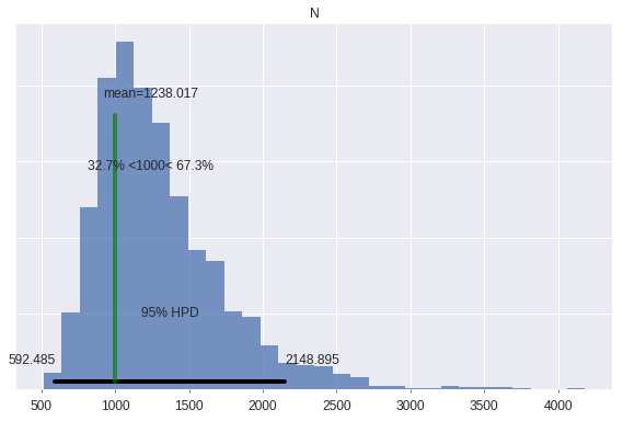
The true population size is well within the 95% credible interval. The posterior estimate of \(N\) could become more accurate by substituting a reasonable upper bound for the prior on \(N\) for the uninformative prior we have used here out of convenience.
The Cormack-Jolly-Seber model
The Cormack-Jolly-Seber model estimates the survival dynamics of individuals in the population by relaxing the third assumption of the Lincoln-Petersen model, that the population is closed. Note that here “survival” does not necessarily correspond to the individual’s death, as it includes individuals that leave the observation area during the study. Despite this subtlety, we will use the convenient terminology of “alive” and “dead” throughout.
For the Cormack-Jolly-Seber and Jolly-Seber models, we follow the notation of Analysis of Capture-Recapture Data by McCrea and Morgan. Additionally, we will use a cormorant data set from the book to illustrate these two models. This data set involves eleven site visits where individuals were given individualized identifying marks. The data are defined below in the form of an \(M\)-array.
T = 10

R = np.array([30, 157, 174, 298, 470, 421, 413, 514, 430, 181])

M = np.zeros((T, T + 1))
M[0, 1:] = [10, 4, 2, 2, 0, 0, 0, 0, 0, 0]
M[1, 2:] = [42, 12, 16, 1, 0, 1, 1, 1, 0]
M[2, 3:] = [85, 22, 5, 5, 2, 1, 0, 1]
M[3, 4:] = [139, 39, 10, 10, 4, 2, 0]
M[4, 5:] = [175, 60, 22, 8, 4, 2]
M[5, 6:] = [159, 46, 16, 5, 2]
M[6, 7:] = [191, 39, 4, 8]
M[7, 8:] = [188, 19, 23]
M[8, 9:] = [101, 55]
M[9, 10] = 84
Here T indicates the number of revisits to the site so there were \(T + 1 = 11\) total visits. The entries of R indicate the number of animals captured and released on each visit.
Rarray([ 30, 157, 174, 298, 470, 421, 413, 514, 430, 181])The entry M[i, j] indicates how many individuals captured on visit \(i\) were first recaptured on visit \(j\). The diagonal of M is entirely zero, since it is not possible to recapture an individual on the same visit as it was released.
M[:4, :4]array([[ 0., 10., 4., 2.],
[ 0., 0., 42., 12.],
[ 0., 0., 0., 85.],
[ 0., 0., 0., 0.]])Of the thirty individuals marked and released on the first visit, ten were recaptured on the second visit, four were recapture on the third visit, and so on.
Capture-recapture data is often given in the form of encounter histories, for example
\[1001000100,\]
which indicates that the individual was first captured on the first visit and recaptured on the fourth and eigth visits. It is straightforward to convert a series of encounter histories to an \(M\)-array. We will discuss encounter histories again at the end of this post.
The parameters of the Cormack-Jolly-Seber model are \(p\), the capture probability, and \(\phi_i\), the probability that an individual that was alive during the \(i\)-th visit is still alive during the \((i + 1)\)-th visit. The capture probability can vary over time in the Cormack-Jolly-Seber model, but we use a constant capture probability here for simplicity.
We again place a uniform prior on \(p\).
with pm.Model() as cjs_model:
    p = pm.Uniform('p', 0., 1.)
We also place a uniform prior on \(\phi_i\).
with cjs_model:
    ϕ = pm.Uniform('ϕ', 0., 1., shape=T)
If \(\nu_{i, j}\) is the probability associated with M[i, j], then
\[ \begin{align*} \nu_{i, j} & = P(\textrm{individual that was alive at visit } i \textrm{ is alive at visit } j) \\ & \times P(\textrm{individual was not captured on visits } i + 1, \ldots, j - 1) \\ & \times P(\textrm{individual is captured on visit } j). \end{align*} \]
From our parameter definitions,
\[P(\textrm{individual that was alive at visit } i \textrm{ is alive at visit } j) = \prod_{k = i}^{j - 1} \phi_k,\]
def fill_lower_diag_ones(x):
    return tt.triu(x) + tt.tril(tt.ones_like(x), k=-1)
with cjs_model:
p_alive = tt.triu(
tt.cumprod(
fill_lower_diag_ones(np.ones_like(M[:, 1:]) * ϕ),
axis=1
)
)\[P(\textrm{individual was not captured at visits } i + 1, \ldots, j - 1) = (1 - p)^{j - i - 1},\]
i = np.arange(T)[:, np.newaxis]
j = np.arange(T + 1)[np.newaxis]

not_cap_visits = np.clip(j - i - 1, 0, np.inf)[:, 1:]
with cjs_model:
p_not_cap = tt.triu(
(1 - p)**not_cap_visits
)and
\[P(\textrm{individual is captured on visit } j) = p.\]
with cjs_model:
    ν = p_alive * p_not_cap * p
The likelihood of the observed recaptures is then
triu_i, triu_j = np.triu_indices_from(M[:, 1:])with cjs_model:
recap_obs = pm.Binomial(
'recap_obs',
M[:, 1:][triu_i, triu_j],
ν[triu_i, triu_j],
observed=M[:, 1:][triu_i, triu_j]
)Finally, some individual released on each occasion are not recaptured again,
R - M.sum(axis=1)array([ 12., 83., 53., 94., 199., 193., 171., 284., 274., 97.])The probability of this event is
\[\chi_i = P(\textrm{released on visit } i \textrm{ and not recaptured again}) = 1 - \sum_{j = i + 1}^T \nu_{i, j}.\]
with cjs_model:
    χ = 1 - ν.sum(axis=1)
The likelihood of the individual that were not recaptured again is
with cjs_model:
    no_recap_obs = pm.Binomial(
        'no_recap_obs',
        R - M.sum(axis=1), χ,
        observed=R - M.sum(axis=1)
    )
Now that the model is fully specified, we sample from its posterior distribution.
with cjs_model:
    cjs_trace = pm.sample(**SAMPLE_KWARGS)
Auto-assigning NUTS sampler...
Initializing NUTS using jitter+adapt_diag...
Multiprocess sampling (3 chains in 3 jobs)
NUTS: [ϕ_interval__, p_interval__]
100%|██████████| 1500/1500 [00:05<00:00, 272.61it/s]Again, the BFMI and energy plot are reasonable.
pm.bfmi(cjs_trace)0.97973424667749842pm.energyplot(cjs_trace);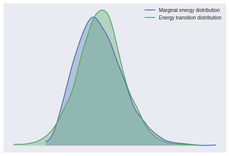
The Gelman-Rubin statistics also indicate convergence.
max(np.max(gr_stats) for gr_stats in pm.gelman_rubin(cjs_trace).values())1.0009026695355843McCrea and Morgan’s book includes a table of maximum likelihood estimates for \(\phi_i\) and \(p\). We verify that our Bayesian estimates are close to these.
ϕ_mle = np.array([0.8, 0.56, 0.83, 0.86, 0.73, 0.69, 0.81, 0.64, 0.46, 0.99])fig, ax = plt.subplots(figsize=(8, 6))
t_plot = np.arange(T) + 1
low, high = np.percentile(cjs_trace['ϕ'], [5, 95], axis=0)
ax.fill_between(
t_plot, low, high,
alpha=0.5, label="90% interval"
);
ax.plot(
t_plot, cjs_trace['ϕ'].mean(axis=0),
label="Posterior expected value"
);
ax.scatter(
t_plot, ϕ_mle,
zorder=5,
c='k', label="Maximum likelihood estimate"
);
ax.set_xlim(1, T);
ax.set_xlabel("$t$");
ax.yaxis.set_major_formatter(PCT_FORMATTER);
ax.set_ylabel(r"$\phi_t$");
ax.legend(loc=2);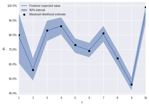
p_mle = 0.51ax = pm.plot_posterior(
cjs_trace, varnames=['p'],
ref_val=p_mle,
lw=0., alpha=0.75
)
ax.set_title("$p$");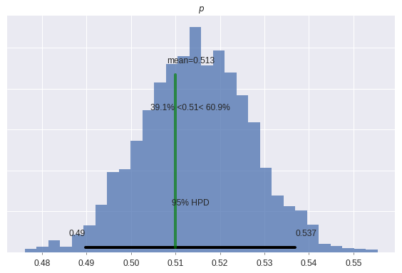
The Jolly-Seber Model
The Jolly-Seber model is an extension of the Cormack-Jolly-Seber model (the fact that the extension is named after fewer people is a bit counterintuitive) that estimates abundance and birth dynamics, in addition to the survival dynamics estimated by the Cormack-Jolly-Seber model. As with the Cormack-Jolly-Seber model where “death” included leaving the site, “birth” includes not just the actual birth of new individuals, but individuals that arrive at the site during the study from elsewhere. Again, despite this subtlety, we will use the convenient terminology of “birth” and “born” throughout.
In order to estimate abundance and birth dynamics, the Jolly-Seber model adds likelihood terms for the first time an individual is captured to the recapture likelihood of the Cormack-Jolly-Seber model. We use the same uniform priors on \(p\) and \(\phi_i\) as in the Cormack-Jolly-Seber model.
with pm.Model() as js_model:
    p = pm.Uniform('p', 0., 1.)
    ϕ = pm.Uniform('ϕ', 0., 1., shape=T)
As with the Lincoln-Petersen model, the Jolly-Seber model estimates the size of the population, including all individuals ever alive during the study period, \(N\). We use the Schwarz-Arnason formulation of the Jolly-Seber model, where each individual has probability \(\beta_i\) of being born into the population between visits \(i\) and \(i + 1\). We place a \(\operatorname{Dirichlet}(1, \ldots, 1)\) prior on these parameters.
with js_model:
    β = pm.Dirichlet('β', np.ones(T), shape=T)
Let \(\Psi_i\) denote the probability that a given individual is alive on visit \(i\) and has not yet been captured before visit \(i\). Then \(\Psi_1 = \beta_0\), since no individuals can have been captured before the first visit, and
\[ \begin{align*} \Psi_{i + 1} & = P(\textrm{the individual was alive and unmarked during visit } i \textrm{ and survived to visit } i + 1) \\ & + P(\textrm{the individual was born between visits } i \textrm{ and } i + 1) \\ & = \Psi_i (1 - p) \phi_i + \beta_i. \end{align*} \]
After writing out the first few terms, we see that this recursion has the closed-form solution
\[\Psi_{i + 1} = \sum_{k = 0}^i \left(\beta_k (1 - p)^{i - k} \prod_{\ell = 1}^{i - k} \phi_{\ell} \right).\]
never_cap_surv_ix = sp.linalg.circulant(np.arange(T))

with js_model:
    p_never_cap_surv = tt.concatenate((
        [1], tt.cumprod((1 - p) * ϕ)[:-1]
    ))

    Ψ = tt.tril(
        β * p_never_cap_surv[never_cap_surv_ix]
    ).sum(axis=1)
The probability that an unmarked individual that is alive at visit \(i\) is captured on visit \(i\) is then \(\Psi_i p\). The probability that an individual is alive at the end of the study period and never captured is \[1 - \sum_{i = 1}^T \Psi_i p.\]
Therefore, the likelihood of the observed first captures is a \((T + 1)\)-dimensional multinomial, where the first \(T\) probabilities are \(\Psi_1 p, \ldots, \Psi_T p\), and the corresponding first \(T\) counts are the observed number of unmarked individuals captured at each visit, \(u_i\). The final probability is
\[1 - \sum_{i = 1}^T \Psi_i p\]
and corresponds to the unobserved number of individuals never captured. Since PyMC3 does not implement such an “incomplete multinomial” distribution, we give a minimal implementation here.
class IncompleteMultinomial(pm.Discrete):
    def __init__(self, n, p, *args, **kwargs):
        """
        n is the total frequency
        p is the vector of probabilities of the observed components
        """
        super(IncompleteMultinomial, self).__init__(*args, **kwargs)
        self.n = n
        self.p = p
        self.mean = n * p.sum() * p,
        self.mode = tt.cast(tt.round(n * p), 'int32')

    def logp(self, x):
        """
        x is the vector of frequences of all but the last components
        """
        n = self.n
        p = self.p

        x_last = n - x.sum()

        return bound(
            factln(n) + tt.sum(x * tt.log(p) - factln(x)) \
                + x_last * tt.log(1 - p.sum()) - factln(x_last),
            tt.all(x >= 0), tt.all(x <= n), tt.sum(x) <= n,
            n >= 0)
As in the Lincoln-Petersen model, we place an improper flat prior (with the appropriate lower bound) on \(N\).
u = np.concatenate(([R[0]], R[1:] - M[:, 1:].sum(axis=0)[:-1]))with js_model:
N = pm.Bound(pm.Flat, lower=u.sum())('N')The likelihood of the observed first captures is therefore
with js_model:
    unmarked_obs = IncompleteMultinomial(
        'unmarked_obs', N, Ψ * p,
        observed=u
    )
The recapture likelihood for the Jolly-Seber model is the same as for the Cormack-Jolly-Seber model.
with js_model:
    p_alive = tt.triu(
        tt.cumprod(
            fill_lower_diag_ones(np.ones_like(M[:, 1:]) * ϕ),
            axis=1
        )
    )
    p_not_cap = tt.triu(
        (1 - p)**not_cap_visits
    )
    ν = p_alive * p_not_cap * p

    recap_obs = pm.Binomial(
        'recap_obs',
        M[:, 1:][triu_i, triu_j], ν[triu_i, triu_j],
        observed=M[:, 1:][triu_i, triu_j]
    )
with js_model:
χ = 1 - ν.sum(axis=1)
no_recap_obs = pm.Binomial(
'no_recap_obs',
R - M.sum(axis=1), χ,
observed=R - M.sum(axis=1)
)Again we sample from the posterior distribution of this model.
with js_model:
    js_trace = pm.sample(**SAMPLE_KWARGS)
Auto-assigning NUTS sampler...
Initializing NUTS using jitter+adapt_diag...
Multiprocess sampling (3 chains in 3 jobs)
NUTS: [N_lowerbound__, β_stickbreaking__, ϕ_interval__, p_interval__]
100%|██████████| 1500/1500 [00:29<00:00, 50.24it/s]Again, the BFMI and energy plot are reasonable.
pm.bfmi(js_trace)0.93076073875335852pm.energyplot(js_trace);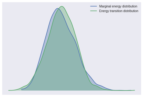
The Gelman-Rubin statistics also indicate convergence.
max(np.max(gr_stats) for gr_stats in pm.gelman_rubin(js_trace).values())1.0051087141503718The posterior expected survival rates are, somewhat surprisingly, still quite similar to the maximum likelihood estimates under the Cormack-Jolly-Seber model.
fig, ax = plt.subplots(figsize=(8, 6))

low, high = np.percentile(js_trace['ϕ'], [5, 95], axis=0)

ax.fill_between(
    t_plot, low, high,
    alpha=0.5, label="90% interval"
);
ax.plot(
    t_plot, js_trace['ϕ'].mean(axis=0),
    label="Posterior expected value"
);

ax.scatter(
    t_plot, ϕ_mle,
    zorder=5,
    c='k', label="Maximum likelihood estimate (CJS)"
);

ax.set_xlim(1, T);
ax.set_xlabel("$t$");

ax.yaxis.set_major_formatter(PCT_FORMATTER);
ax.set_ylabel(r"$\phi_t$");

ax.legend(loc="upper center");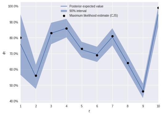
The following plot shows the estimated birth dynamics.
fig, ax = plt.subplots(figsize=(8, 6))

low, high = np.percentile(js_trace['β'], [5, 95], axis=0)

ax.fill_between(
    t_plot - 1, low, high,
    alpha=0.5, label="90% interval"
);
ax.plot(
    t_plot - 1, js_trace['β'].mean(axis=0),
    label="Posterior expected value"
);

ax.set_xlim(0, T - 1);
ax.set_xlabel("$t$");

ax.yaxis.set_major_formatter(PCT_FORMATTER);
ax.set_ylabel(r"$\beta_t$");

ax.legend(loc=2);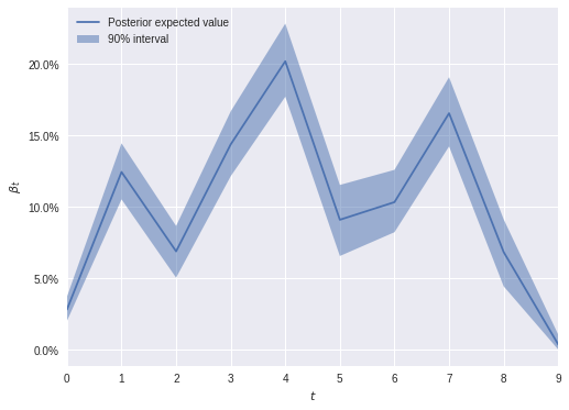
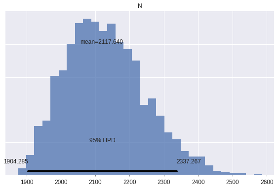
The posterior expected population size is about 30% larger than the number of distinct individuals marked.
js_trace['N'].mean() / u.sum()1.2951923918464066pm.plot_posterior(
js_trace, varnames=['N'],
lw=0., alpha=0.75
);
Now that we have estimated these three models, we return briefly to the topic of \(M\)-arrays versus encounter histories. While \(M\)-arrays are a convienent summary of encounter histories, they do not lend themselves to common extensions of these models to include individual random effects, trap-dependent recapture, etc. as readily as encounter histories. Two possibile approaches to include such effects are:
- Use likelihoods for the (Cormack-)Jolly-Seber models based on encounter histories, which are a bit more complex than those based on \(M\)-arrays.
- Individual \(M\)-arrays: transform each individual’s account history into an \(M\)-array an stack them into a three-dimensional array of \(M\)-arrays.
We may explore one (or both) of these approaches in a future post.
Thanks to Eric Heydenberk for his feedback on a early draft of this post.
This post is available as a Jupyter notebook here.