A Fair Price for Darth Vader's Meditation Chamber? A Lego Price Analysis
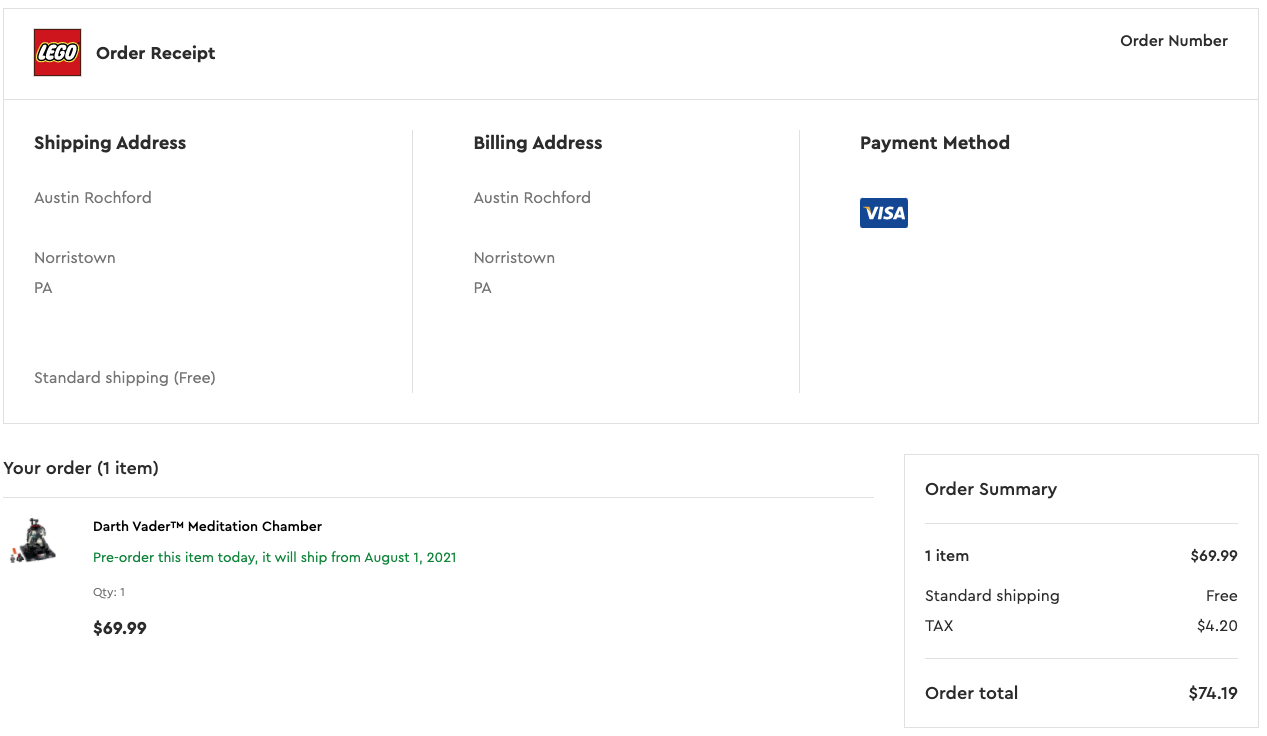
Earlier this week I was taking a break from work and browsing lego.com (as one does), and came across Darth Vader’s Meditation Chamber (75296), which is newly available for preorder.
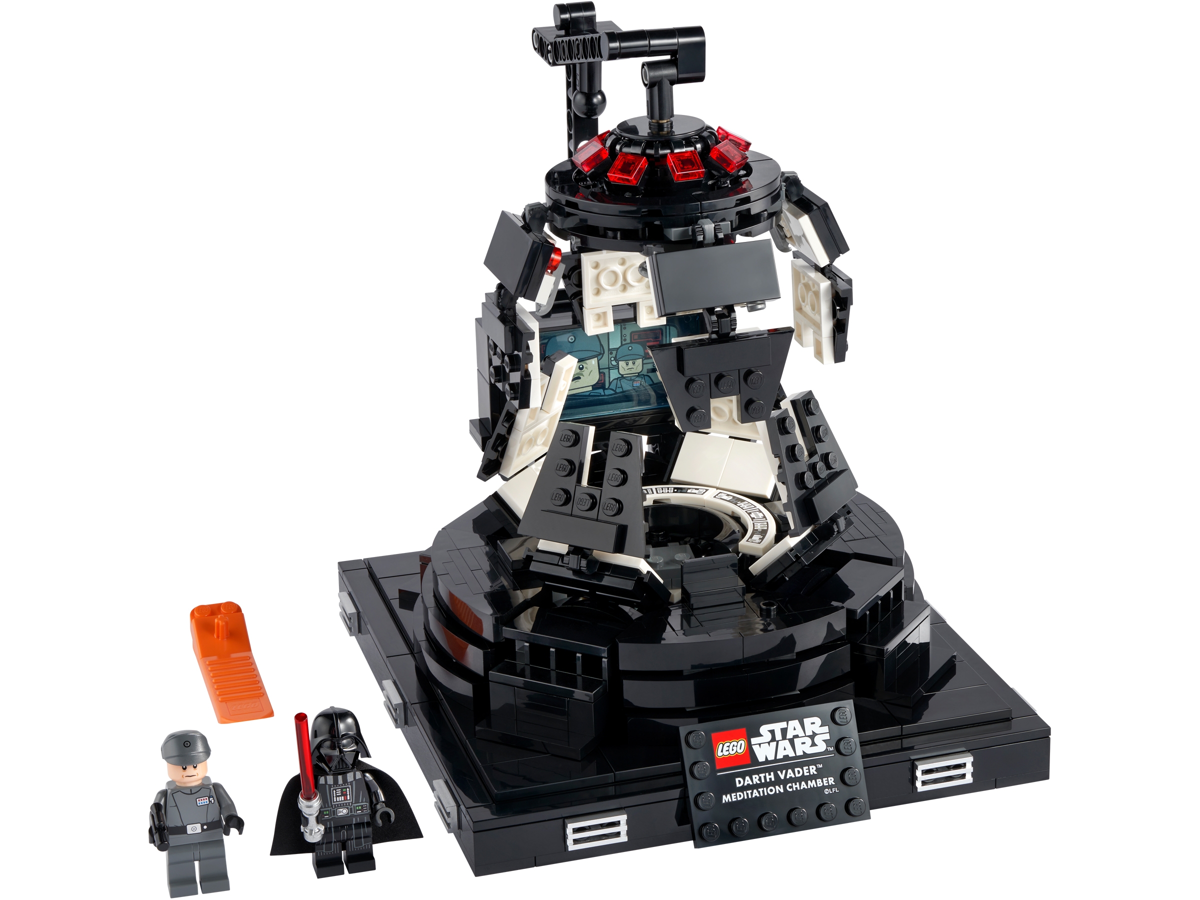
My first thought was “this looks nice, but $69.99 feels a bit steep for 663 pieces.” Being both a Lego and data nerd, I decided to see how good or bad this price actually is compared to other sets.
|
|
|
|
I searched for a freely available source of data on Lego set prices, but didn’t find any that were suitable to answer my question. After a few hours of frustration, I wrote a small Python script using Beautiful Soup to scrape brickset.com’s historical data on Lego sets dating back to 1980. Out of respect for the hard and excellent work of the Brickset team, I won’t be sharing the scraper code, but I have made the data set (scraped on June 1, 2021) publicly available. This is the first post in a series analyzing this data.
DATA_URL = 'https://austinrochford.com/resources/lego/brickset_01011980_06012021.csv.gz'First we make some standard Python imports and load the data.
%matplotlib inlineimport datetime
from functools import reduce
from warnings import filterwarningsfrom matplotlib import MatplotlibDeprecationWarning, pyplot as plt
import numpy as np
import pandas as pd
import seaborn as snsfilterwarnings('ignore', category=MatplotlibDeprecationWarning)plt.rcParams['figure.figsize'] = (8, 6)
sns.set(color_codes=True)def to_datetime(year):
return np.datetime64(f"{round(year)}-01-01")full_df = (pd.read_csv(DATA_URL,
usecols=[
"Year released", "Set number",
"Name", "Set type", "Theme", "Subtheme",
"Pieces", "RRP"
])
.dropna(subset=[
"Year released", "Set number",
"Name", "Set type", "Theme",
"Pieces", "RRP"
]))
full_df["Year released"] = full_df["Year released"].apply(to_datetime)
full_df = (full_df.set_index(["Year released", "Set number"])
.sort_index())full_df.head()| Name | Set type | Theme | Pieces | RRP | Subtheme | ||
|---|---|---|---|---|---|---|---|
| Year released | Set number | ||||||
| 1980-01-01 | 1041-2 | Educational Duplo Building Set | Normal | Dacta | 68.0 | 36.50 | NaN |
| 1075-1 | LEGO People Supplementary Set | Normal | Dacta | 304.0 | 14.50 | NaN | |
| 1101-1 | Replacement 4.5V Motor | Normal | Service Packs | 1.0 | 5.65 | NaN | |
| 1123-1 | Ball and Socket Couplings & One Articulated Joint | Normal | Service Packs | 8.0 | 16.00 | NaN | |
| 1130-1 | Plastic Folder for Building Instructions | Normal | Service Packs | 1.0 | 14.00 | NaN |
full_df.tail()| Name | Set type | Theme | Pieces | RRP | Subtheme | ||
|---|---|---|---|---|---|---|---|
| Year released | Set number | ||||||
| 2021-01-01 | 80022-1 | Spider Queen’s Arachnoid Base | Normal | Monkie Kid | 1170.0 | 119.99 | Season 2 |
| 80023-1 | Monkie Kid’s Team Dronecopter | Normal | Monkie Kid | 1462.0 | 149.99 | Season 2 | |
| 80024-1 | The Legendary Flower Fruit Mountain | Normal | Monkie Kid | 1949.0 | 169.99 | Season 2 | |
| 80106-1 | Story of Nian | Normal | Seasonal | 1067.0 | 79.99 | Chinese Traditional Festivals | |
| 80107-1 | Spring Lantern Festival | Normal | Seasonal | 1793.0 | 119.99 | Chinese Traditional Festivals |
Most of the fields are fairly self-explanatory. RRP is the recommended retail price of the set in dollars.
For fun, I have also exported my Lego collection from Brickset and load it now.
MY_COLLECTION_URL = 'https://austinrochford.com/resources/lego/Brickset-MySets-owned-20210602.csv'my_df = pd.read_csv(MY_COLLECTION_URL)my_df.indexIndex(['8092-1', '10221-1', '10266-1', '10281-1', '10283-1', '21309-1',
'21312-1', '21320-1', '21321-1', '31091-1', '40174-1', '40268-1',
'40391-1', '40431-1', '40440-1', '41602-1', '41608-1', '41609-1',
'41628-1', '75030-1', '75049-1', '75074-1', '75075-1', '75093-1',
'75099-1', '75136-1', '75137-1', '75138-1', '75162-1', '75176-1',
'75187-1', '75229-1', '75243-1', '75244-1', '75248-1', '75254-1',
'75255-1', '75263-1', '75264-1', '75266-1', '75267-1', '75269-1',
'75273-1', '75277-1', '75278-1', '75283-1', '75292-1', '75297-1',
'75302-1', '75306-1', '75308-1', '75317-1', '75318-1'],
dtype='object')We add a column to full_df indicating whether or not I own the set represented by each row.
full_df["austin"] = (full_df.index
                            .get_level_values("Set number")
                            .isin(my_df.index))
Exploratory Data Analysis
First we check for any missing data.
full_df.isnull().mean()Name 0.000000
Set type 0.000000
Theme 0.000000
Pieces 0.000000
RRP 0.000000
Subtheme 0.241825
austin 0.000000
dtype: float64About a quarter of the sets do not have a Subtheme, but each set has data for every other column. We see below that most sets are classified as “normal” building sets, but there are some books and other types of sets present in the data.
ax = (full_df["Set type"]
             .value_counts(ascending=True)
             .plot(kind='barh'))

ax.set_xscale('log');
ax.set_xlabel("Number of sets");

ax.set_ylabel("Set type");
For simplicity, we will focus only on “normal” sets.
FILTERS = [full_df["Set type"] == "Normal"]df = full_df[reduce(np.logical_and, FILTERS)]We still have information on over 8,000 sets.
df["Pieces"].describe()count 8163.000000
mean 265.848095
std 489.269642
min 1.000000
25% 34.000000
50% 102.000000
75% 310.000000
max 11695.000000
Name: Pieces, dtype: float64The set with the most pieces is the recently released World Map, (31203-1).
df.loc[df["Pieces"].idxmax()]Name World Map
Set type Normal
Theme Art
Pieces 11695.0
RRP 249.99
Subtheme Miscellaneous
austin False
Name: (2021-01-01 00:00:00, 31203-1), dtype: object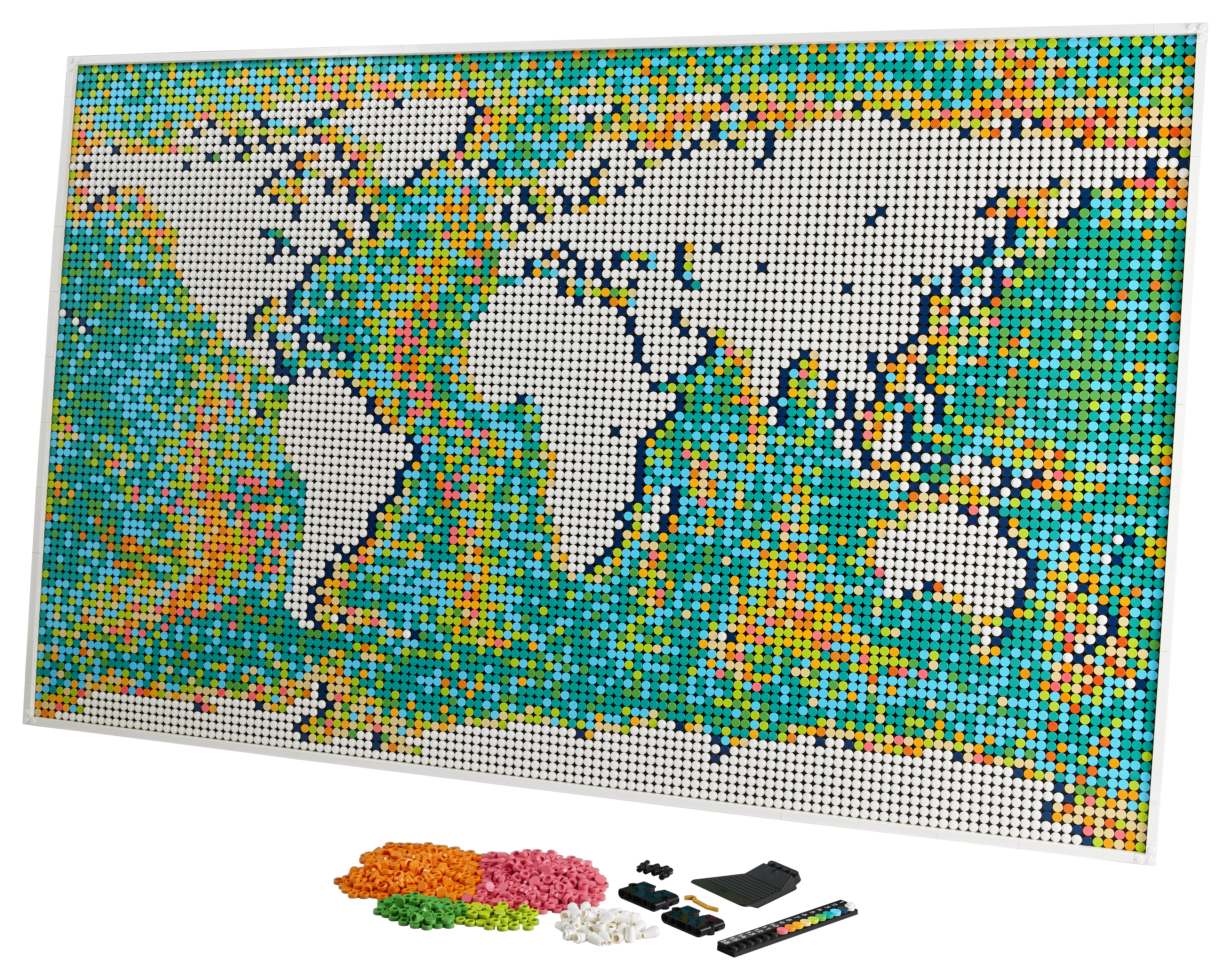
I love the idea of a Lego world map, but I’m not in love with the ocean color, so I’ll probably pass on this beast.
We see below that here are many sets with very few pieces (presumably replacement parts, minifigures, and promotional sets).
max_pieces = df["Pieces"].max()
plt_max_pieces = 1.1 * max_pieces

ax = sns.kdeplot(data=full_df, x="Pieces",
                 label="All sets")
sns.rugplot(data=full_df, x="Pieces",
            c='k', alpha=0.1, ax=ax);

THRESHES = [1, 10, 25, 50, 100]

for thresh in THRESHES:
    sns.kdeplot(data=full_df[full_df["Pieces"] > thresh],
                x="Pieces",
                clip=(thresh, plt_max_pieces),
                label=f"Sets with more\nthan {thresh} pieces",
                ax=ax);

ax.set_xscale('log');
ax.set_xticks(THRESHES + [10**3, 10**4])
ax.set_xlim(0.9, plt_max_pieces);

ax.set_yticks([]);
ax.legend();
We filter our analysis to sets with more than 10 pieces.
FILTERS.append(full_df["Pieces"] > 10)df = full_df[reduce(np.logical_and, FILTERS)]Note that by using FILTERS.append the order of execution of cells in this notebook becomes very important (notebooks are bad, etc., but I love them anyway).
We now examine the distribution of sets across themes.
(df["Theme"]
   .value_counts()
   .describe())
count 134.000000
mean 52.992537
std 94.157163
min 1.000000
25% 7.000000
50% 19.000000
75% 52.500000
max 556.000000
Name: Theme, dtype: float64n_theme = df["Theme"].nunique()
N_THEME_PLOTS = 12
N_THEME_COLS = 2
n_theme_rows = N_THEME_PLOTS // N_THEME_COLS
n_themes_per_plot = int(np.ceil(n_theme / N_THEME_PLOTS))fig, axes = plt.subplots(nrows=n_theme_rows, ncols=N_THEME_COLS,
sharex=True, sharey=False,
figsize=(16, n_theme_rows * 6))
theme_ct = df["Theme"].value_counts()
for i, ax in zip(range(0, n_theme, n_themes_per_plot),
axes.flatten()):
(theme_ct.iloc[i:i + n_themes_per_plot]
.plot(kind='barh', ax=ax));
ax.set_xscale('log');
ax.set_xlabel("Number of sets");
ax.invert_yaxis();
ax.set_ylabel("Theme");
fig.tight_layout();
Unsurprisingly, the Star Wars theme has the most sets historically. That Duplo comes in second is interesting. We filter out Duplo sets, service pack, and bulk brick sets from our analysis.
FILTERS.append(full_df["Theme"] != "Duplo")
FILTERS.append(full_df["Theme"] != "Service Packs")
FILTERS.append(full_df["Theme"] != "Bulk Bricks")
df = full_df[reduce(np.logical_and, FILTERS)]Set Price
We now turn to the question that prompted this work, whether or not Darth Vader’s Meditation Chamber is overpriced. Our set data spans 1980-2021, and we see that the number of sets released has been increasing fairly steadily over the years.
ax = (df.index
        .get_level_values("Year released")
        .value_counts()
        .sort_index()
        .plot())

ax.set_xlabel("Year released");
ax.set_ylabel("Number of sets");
Since the data spans more than 40 years, it is important to adjust for inflation. We use the Consumer Price Index for All Urban Consumers: All Items in U.S. City Average from the U.S. Federal Reserve to adjust for inflation.
CPI_URL = 'https://austinrochford.com/resources/lego/CPIAUCNS202100401.csv'years = pd.date_range('1979-01-01', '2021-01-01', freq='Y') \
+ datetime.timedelta(days=1)
cpi_df = (pd.read_csv(CPI_URL, index_col="DATE", parse_dates=["DATE"])
.loc[years])
cpi_df["to2021"] = cpi_df.loc["2021-01-01"] / cpi_dffig, (cpi_ax, factor_ax) = plt.subplots(ncols=2, sharex=True, sharey=False,
figsize=(16, 6))
cpi_df["CPIAUCNS"].plot(ax=cpi_ax);
cpi_ax.set_xlabel("Year");
cpi_ax.set_ylabel("CPIAUCNS");
cpi_df["to2021"].plot(ax=factor_ax);
factor_ax.set_xlabel("Year");
factor_ax.set_ylabel("Inflation multiple to 2021 dollars");
fig.tight_layout();
We now add a column RRP2021, which is RRP adjusted to 2021 dollars.
full_df["RRP2021"] = (pd.merge(full_df, cpi_df,
                               left_on=["Year released"],
                               right_index=True)
                        .apply(lambda df: df["RRP"] * df["to2021"],
                               axis=1))
df = full_df[reduce(np.logical_and, FILTERS)]Here we plot the most obvious relationship pertinent to my initial question about Darth Vader’s Meditation Chamber, price versus number of pieces.
ax = sns.scatterplot(x="Pieces", y="RRP2021", data=df, alpha=0.1)
sns.scatterplot(x="Pieces", y="RRP2021",
                data=df[df["austin"] == True],
                alpha=0.5, label="My sets");

ax.set_xscale('log');

ax.set_yscale('log');
ax.set_ylabel("Retail price (2021 $)");
The relationship is fairly linear on a log-log scale, which will be important in subsequent posts when we introduce more complex statistical models. The sets in my collection are highlighted in this plot.
We can also highlight certain themes of interest to see where the sets from those themes fall.
PLOT_THEMES = [
    "Creator Expert",
    "Disney",
    "Star Wars",
    "Harry Potter",
    "Marvel Super Heroes",
    "Ninjago",
    "City",
    "Space",
    "Jurassic World"
]
grid = sns.relplot(x="Pieces", y="RRP2021", col="Theme",
data=df[df["Theme"].isin(PLOT_THEMES)],
color='C1', alpha=0.5, col_wrap=3, zorder=5)
for ax in grid.axes.flatten():
sns.scatterplot(x="Pieces", y="RRP2021", data=df,
color='C0', alpha=0.05,
ax=ax);
ax.set_xscale('log');
ax.set_yscale('log');
ax.set_ylabel("Retail price (2021 $)");
There are some interesting relationships here.
- Space sets seem to be more expensive per piece than average.
- Star Wars, City, Harry Potter, and Jurassic World sets seem to be fairly uniformly distributed around the average price per piece.
- Marvel Super Heroes and Ninjago seem to be less expensive per piece than average.
- Creator Expert sets have many pieces, which makes perfect sense.
We’ll dig deeper into these observations in a subsequent post.
We now add a DPP2021 column to the data frame which represents the set’s price per piece in 2021 dollars.
full_df["DPP2021"] = (df["RRP2021"]
                        .div(df["Pieces"])
                        .rename("DPP2021"))
df = full_df[reduce(np.logical_and, FILTERS)]In order to decide whether or not Darth Vader’s Meditation Chamber is overpriced, we look at the percentile of its adjusted price per piece in various populations of sets.
VADER_MEDITATION = "75296-1"We see that this set is in the 25th percentile of adjusted price per piece among all sets, and the 13th percentile among Star Wars sets.
(df["DPP2021"]
   .lt(df["DPP2021"]
         .xs(VADER_MEDITATION, level="Set number")
         .values[0])
.mean())0.25019669551534224(df["DPP2021"]
[df["Theme"] == "Star Wars"]
.lt(df["DPP2021"]
.xs(VADER_MEDITATION, level="Set number")
.values[0])
.mean())0.13309352517985612Its adjusted price per piece is near the median for my collection (apparently I’m relatively cheap), but still nowhere near a bad value by this metric.
(df[df["austin"] == True]
   ["DPP2021"]
   .lt(df["DPP2021"]
         .xs(VADER_MEDITATION, level="Set number")
         .values[0])
.mean())0.46153846153846156ax = sns.scatterplot(x="Pieces", y="RRP2021", data=df,
color='C0', alpha=0.05,
label="All sets");
sns.scatterplot(x="Pieces", y="RRP2021",
data=df[df["Theme"] == "Star Wars"],
color='C1', alpha=0.5,
label="Star wars sets",
ax=ax);
sns.scatterplot(x="Pieces", y="RRP2021",
data=df[df["austin"] == True],
color='C2', alpha=0.5,
label="My sets",
ax=ax);
ax.scatter(df["Pieces"].xs(VADER_MEDITATION, level="Set number"),
df["RRP2021"].xs(VADER_MEDITATION, level="Set number"),
color="C3", s=150, marker='D', alpha=0.9,
label=f"Darth Vader's Meditation Chamber ({VADER_MEDITATION})");
ax.set_xscale('log');
ax.set_yscale('log');
ax.set_ylabel("Retail price (2021 $)");
ax.legend(loc='upper left');
As an apology to my Lego overlords, I preordered Darth Vader’s Meditation Chamber after doing this analysis.
It is also interesting to examine how the adjusted price per piece has changed over time.
ax = sns.lineplot(x="Year released", y="DPP2021", data=df,
                  color='k')

ax.set_ylim(10**-1, 2);
ax.set_yscale('log');
ax.set_ylabel("Price per piece (2021 $)");
It seems that the adjusted price per piece has been steadily decreasing over time. Presumably Lego has been optimizing their manufacturing processes to be more efficient over the years and has passed some of the reduction in costs onto we consumers. Lego has likely improved set pricing over time as they have accumulated historical data on sales of past sets.
When we break this timeseries down by theme we see a general convergence of the price per piece to the average across our themes of interest.
ax = sns.lineplot(x="Year released", y="DPP2021", data=df,
                  color='k', label="All")
sns.lineplot(x="Year released", y="DPP2021", hue="Theme",
             data=df[df["Theme"].isin(PLOT_THEMES)],
             ax=ax);

ax.set_ylim(10**-1, 2);
ax.set_yscale('log');
ax.set_ylabel("Price per piece (2021 $)");
Future posts in this series will introduce more complex statistical models for this data and use them to explore these trends and more structure in the data.
This post is available as a Jupyter notebook here. The Docker environment that this post was written in is available here.
%load_ext watermark
%watermark -n -u -v -iv
Last updated: Thu Jun 03 2021
Python implementation: CPython
Python version : 3.8.8
IPython version : 7.22.0
matplotlib: 3.4.1
numpy : 1.20.2
pandas : 1.2.3
seaborn : 0.11.1