Maximum Likelihood Estimation of Custom Models in Python with StatsModels
Maximum likelihood estimation is a common method for fitting statistical models. In Python, it is quite possible to fit maximum likelihood models using just scipy.optimize. Over time, however, I have come to prefer the convenience provided by statsmodels’ GenericLikelihoodModel. In this post, I will show how easy it is to subclass GenericLikelihoodModel and take advantage of much of statsmodels’ well-developed machinery for maximum likelihood estimation of custom models.
Zero-inflated Poisson models
The model we use for this demonstration is a zero-inflated Poisson model. This is a model for count data that generalizes the Poisson model by allowing for an overabundance of zero observations.
The model has two parameters, \(\pi\), the proportion of excess zero observations, and \(\lambda\), the mean of the Poisson distribution. We assume that observations from this model are generated as follows. First, a weighted coin with probability \(\pi\) of landing on heads is flipped. If the result is heads, the observation is zero. If the result is tails, the observation is generated from a Poisson distribution with mean \(\lambda\). Note that there are two ways for an observation to be zero under this model:
- the coin is heads, and
- the coin is tails, and the sample from the Poisson distribution is zero.
If \(X\) has a zero-inflated Poisson distribution with parameters \(\pi\) and \(\lambda\), its probability mass function is given by
\[\begin{align*} P(X = 0) & = \pi + (1 - \pi)\ e^{-\lambda} \\ P(X = x) & = (1 - \pi)\ e^{-\lambda}\ \frac{\lambda^x}{x!} \textrm{ for } x > 0. \end{align*}\]
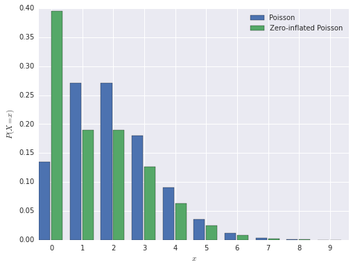
In this post, we will use the parameter values \(\pi = 0.3\) and \(\lambda = 2\). The probability mass function of the zero-inflated Poisson distribution is shown below, next to a normal Poisson distribution, for comparison.
from __future__ import division

from matplotlib import  pyplot as plt
import numpy as np
from scipy import stats
import seaborn as sns
from statsmodels.base.model import GenericLikelihoodModel

np.random.seed(123456789)
pi = 0.3
lambda_ = 2.def zip_pmf(x, pi=pi, lambda_=lambda_):
if pi < 0 or pi > 1 or lambda_ <= 0:
return np.zeros_like(x)
else:
return (x == 0) * pi + (1 - pi) * stats.poisson.pmf(x, lambda_)
Maximum likelihood estimation
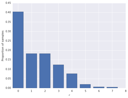
First we generate 1,000 observations from the zero-inflated model.
N = 1000

inflated_zero = stats.bernoulli.rvs(pi, size=N)
x = (1 - inflated_zero) * stats.poisson.rvs(lambda_, size=N)
We are now ready to estimate \(\pi\) and \(\lambda\) by maximum likelihood. To do so, we define a class that inherits from statsmodels’ GenericLikelihoodModel as follows.
class ZeroInflatedPoisson(GenericLikelihoodModel):
    def __init__(self, endog, exog=None, **kwds):
        if exog is None:
            exog = np.zeros_like(endog)

        super(ZeroInflatedPoisson, self).__init__(endog, exog, **kwds)

    def nloglikeobs(self, params):
        pi = params[0]
        lambda_ = params[1]

        return -np.log(zip_pmf(self.endog, pi=pi, lambda_=lambda_))

    def fit(self, start_params=None, maxiter=10000, maxfun=5000, **kwds):
        if start_params is None:
            lambda_start = self.endog.mean()
            excess_zeros = (self.endog == 0).mean() - stats.poisson.pmf(0, lambda_start)

            start_params = np.array([excess_zeros, lambda_start])

        return super(ZeroInflatedPoisson, self).fit(start_params=start_params,
                                                    maxiter=maxiter, maxfun=maxfun, **kwds)
The key component of this class is the method nloglikeobs, which returns the negative log likelihood of each observed value in endog. Secondarily, we must also supply reasonable initial guesses of the parameters in fit. Obtaining the maximum likelihood estimate is now simple.
model = ZeroInflatedPoisson(x)
results = model.fit()
Optimization terminated successfully.
Current function value: 1.586641
Iterations: 37
Function evaluations: 70We see that we have estimated the parameters fairly well.
pi_mle, lambda_mle = results.params

pi_mle, lambda_mle
(0.31542487710071976, 2.0451304204850853)There are many advantages to buying into the statsmodels ecosystem and subclassing GenericLikelihoodModel. The already-written statsmodels code handles storing the observations and the interaction with scipy.optimize for us. (It is possible to control the use of scipy.optimize through keyword arguments to fit.)
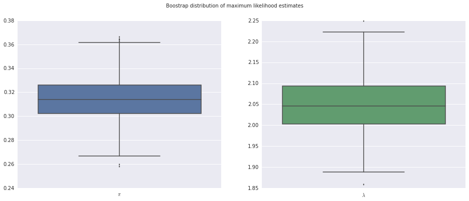
We also gain access to many of statsmodels’ built in model analysis tools. For example, we can use bootstrap resampling to estimate the variation in our parameter estimates.
boot_mean, boot_std, boot_samples = results.bootstrap(nrep=500, store=True)
boot_pis = boot_samples[:, 0]
boot_lambdas = boot_samples[:, 1]
The next time you are fitting a model using maximum likelihood, try integrating with statsmodels to take advantage of the significant amount of work that has gone into its ecosystem.