Monotonic Effects in PyMC3
Last week I came across the following tweet from Paul Bürkner about a paper he coauthored about including ordinal predictors in Bayesian regression models, and I thought the approach was very clever.
Have you ever wondered how to handle ordinal predictors in your regression models? We propose a simple and intuitive method that is readily available via #brms and @mcmc_stan: https://t.co/dKg4AphvsG
— Paul Bürkner (@paulbuerkner) November 2, 2018
The code in the paper uses brms and Stan to illustrate these concepts. In this post I’ll be replicating some of the paper’s analysis in Python and PyMC3, mostly for my own edification.
%matplotlib inlinefrom itertools import productimport arviz as az
from matplotlib import pyplot as plt
import numpy as np
import pandas as pd
import pymc3 as pm
from rpy2.robjects import pandas2ri, r
import seaborn as sns
from theano import sharedsns.set()The paper uses data from the ordPens R package, which we download and load into a Pandas DataFrame.
%%bash
if [[ ! -e ~/data/ordPens ]];
then
    mkdir -p data
    wget -q -O data/ordPens_0.3-1.tar.gz ~/data/ https://cran.r-project.org/src/contrib/ordPens_0.3-1.tar.gz
    tar xzf data/ordPens_0.3-1.tar.gz -C data
fi!ls data/ordPens/data/ICFCoreSetCWP.RDatapandas2ri.activate()
r.load('data/ordPens/data/ICFCoreSetCWP.RData');
all_df = r['ICFCoreSetCWP']all_df.head()| b1602 | b122 | b126 | b130 | b134 | b140 | b147 | b152 | b164 | b180 | … | e450 | e455 | e460 | e465 | e570 | e575 | e580 | e590 | s770 | phcs | |
|---|---|---|---|---|---|---|---|---|---|---|---|---|---|---|---|---|---|---|---|---|---|
| 1 | 0 | 1 | 2 | 1 | 1 | 0 | 0 | 2 | 0 | 0 | … | 4 | 0 | 0 | 0 | 3 | 3 | 4 | 3 | 0 | 44.33 |
| 2 | 3 | 2 | 2 | 3 | 3 | 2 | 3 | 3 | 3 | 1 | … | 3 | 3 | 2 | 2 | 2 | 2 | 2 | 2 | 2 | 21.09 |
| 3 | 0 | 1 | 2 | 1 | 1 | 0 | 1 | 2 | 0 | 0 | … | 4 | 0 | 0 | 0 | 3 | 3 | 4 | 0 | 0 | 41.74 |
| 4 | 0 | 0 | 0 | 2 | 1 | 0 | 0 | 0 | 0 | 0 | … | 2 | 2 | -1 | 0 | 0 | 2 | 2 | 1 | 1 | 33.96 |
| 5 | 0 | 0 | 0 | 0 | 0 | 0 | 0 | 0 | 0 | 0 | … | 1 | 0 | 0 | 0 | 0 | 0 | 0 | 0 | 0 | 46.29 |
5 rows × 68 columns
The variable of interest here is phcs, which is a subjective physical health score. The predictors we are interested in are d450 and d455.
df = all_df[['d450', 'd455', 'phcs']]df.head()| d450 | d455 | phcs | |
|---|---|---|---|
| 1 | 0 | 2 | 44.33 |
| 2 | 3 | 3 | 21.09 |
| 3 | 0 | 2 | 41.74 |
| 4 | 3 | 2 | 33.96 |
| 5 | 0 | 0 | 46.29 |
These predictors are ratings on a five-point scale (0-4) of the patient’s impairment while walking (d450) and moving around (d455). For more information on this data, consult the ordPens documentation.
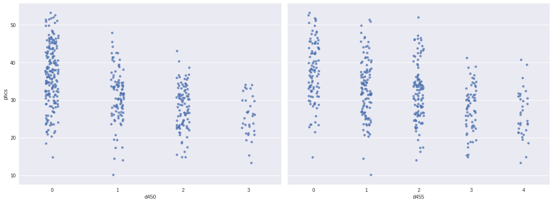
The following plots show a fairly strong monotonic relationship between d450, d455, and phcs.
fig, (d450_ax, d455_ax) = plt.subplots(ncols=2, sharey=True, figsize=(16, 6))

sns.stripplot('d450', 'phcs', data=df,
              jitter=0.1, color='C0', alpha=0.75,
              ax=d450_ax);
sns.stripplot('d455', 'phcs', data=df,
              jitter=0.1, color='C0', alpha=0.75,
              ax=d455_ax);

d455_ax.set_ylabel("");
fig.tight_layout();
The big idea of the paper is to include monotonic effects due to these ordinal predictors as follows. A scalar \(b \sim N(0, 10^2)\) parameterizes the overall strength and direction of the relationship, and a Dirichlet vector \(\xi \sim \textrm{Dirichlet}(1, \ldots, 1)\) encodes how much of \(b\) is gained at each level. The parameters \(b\) and \(\xi\) are combined into
\[mo(i) = b \sum_{k = 0}^i \xi_k\]
which can be included as a term in a regression model. It is evident that if \(i < j\) then \(mo(i) \leq mo(j)\) since
\[mo(j) - mo(i) = b \sum_{k = i + 1}^j \xi_k \geq 0\]
and therefore the effect of this term will be monotonic as desired.
The following function constructs this distribution in PyMC3.
def monotonic_prior(name, n_cat):
    b = pm.Normal(f'b_{name}', 0., 10.)
    ξ = pm.Dirichlet(f'ξ_{name}', np.ones(n_cat))

    return pm.Deterministic(f'mo_{name}', b * ξ.cumsum())
With this notation in hand, our model is
\[ \begin{align*} \mu_i & = \beta_0 + mo_{\textrm{d450}}(j_i) + mo_{\textrm{d455}}(k_i) \\ \beta_0 & \sim N(0, 10^2) \\ y_i & \sim N(\mu_i, \sigma^2) \\ \sigma & \sim \textrm{HalfNormal}(5^2) \end{align*} \]
where \(j_i\) and \(k_i\) are the level of d450 and d455 for the \(i\)-th patient respectively and \(y_i\) is that patient’s phcs score.
We now express this model in PyMC3.
d450 = df['d450'].values
d450_cats = np.unique(d450)
d450_n_cat = d450_cats.size
d450_ = shared(d450)

d455 = df['d455'].values
d455_cats = np.unique(d455)
d455_n_cat = d455_cats.size
d455_ = shared(d455)

phcs = df['phcs'].values
with pm.Model() as model:
β0 = pm.Normal('β0', 0., 10.)
mo_d450 = monotonic_prior('d450', d450_n_cat)
mo_d455 = monotonic_prior('d455', d455_n_cat)
μ = β0 + mo_d450[d450_] + mo_d455[d455_]
σ = pm.HalfNormal('σ', 5.)
phcs_obs = pm.Normal('phcs', μ, σ, observed=phcs)We now sample from the model’s posterior distribution.
CHAINS = 3
SEED = 934520 # from random.org

SAMPLE_KWARGS = {
    'draws': 1000,
    'tune': 1000,
    'chains': CHAINS,
    'random_seed': list(SEED + np.arange(CHAINS))
}
with model:
trace = pm.sample(**SAMPLE_KWARGS)Auto-assigning NUTS sampler...
Initializing NUTS using jitter+adapt_diag...
Multiprocess sampling (3 chains in 2 jobs)
NUTS: [σ, ξ_d455, b_d455, ξ_d450, b_d450, β0]
Sampling 3 chains: 100%|██████████| 6000/6000 [00:41<00:00, 145.59draws/s]
The number of effective samples is smaller than 25% for some parameters.We use arviz to check the performance of our sampler.
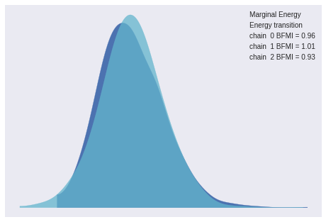
inf_data = az.convert_to_inference_data(trace)The energy plot, BFMI, and Gelman-Rubin statistics show no cause for concern.
az.plot_energy(inf_data);
az.gelman_rubin(inf_data).max()<xarray.Dataset>
Dimensions: ()
Data variables:
β0 float64 1.0
b_d450 float64 1.0
b_d455 float64 1.0
ξ_d450 float64 1.0
mo_d450 float64 1.0
ξ_d455 float64 1.0
mo_d455 float64 1.0
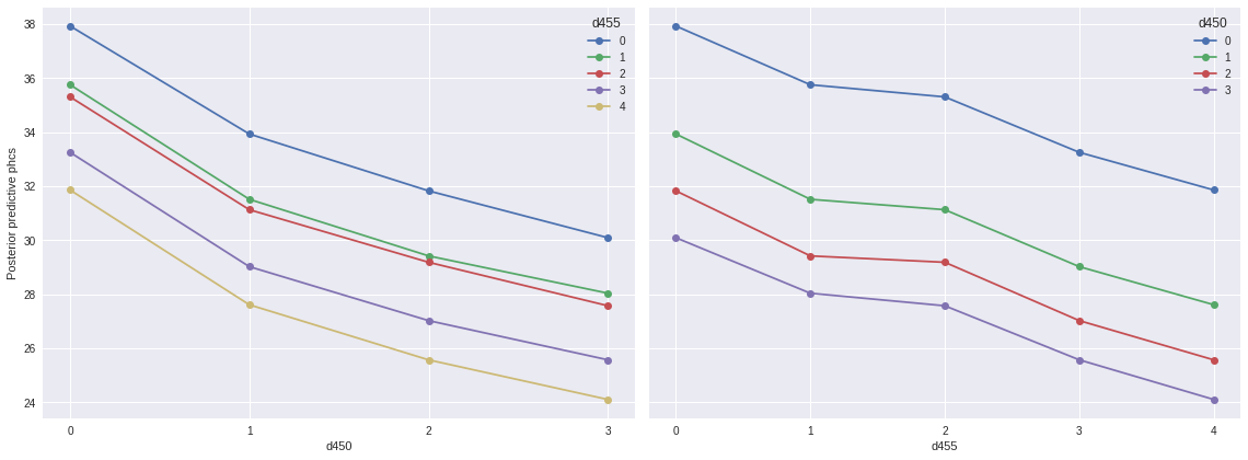
σ float64 1.0We now sample from the model’s posterior predictive distribution and visualize the results.
pp_d450, pp_d455 = np.asarray(list(zip(*product(d450_cats, d455_cats))))

d450_.set_value(pp_d450)
d455_.set_value(pp_d455)
with model:
pp_trace = pm.sample_posterior_predictive(trace)100%|██████████| 3000/3000 [00:07<00:00, 388.49it/s]pp_df = pd.DataFrame({
'd450': pp_d450,
'd455': pp_d455,
'pp_phcs_mean': pp_trace['phcs'].mean(axis=0)
})The important feature of this encoding of ordinal predictors is that the \(\xi\) parameters allow different levels of the predictor to contribute to result in a different change in the effect, which is in contrast to what happens when these are included as linear predictors, which is quite common in the literature.
REF_CAT = 1fig, (d450_ax, d455_ax) = plt.subplots(ncols=2, sharey=True, figsize=(16, 6))
(pp_df.pivot_table('pp_phcs_mean', 'd450', 'd455')
.plot(marker='o', ax=d450_ax));
d450_ax.set_xticks(d450_cats);
d450_ax.set_ylabel("Posterior predictive phcs");
(pp_df.pivot_table('pp_phcs_mean', 'd455', 'd450')
.plot(marker='o', ax=d455_ax));
d455_ax.set_xticks(d455_cats);
fig.tight_layout();
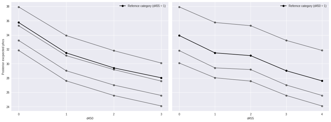
The following plot corresponds to Figure 3 in the original paper, and the dark lines agree with the mean in that figure quite well.
fig, (d450_ax, d455_ax) = plt.subplots(ncols=2, sharey=True, figsize=(16, 6))

(pp_df[pp_df['d455'] != REF_CAT]
      .pivot_table('pp_phcs_mean', 'd450', 'd455')
      .plot(marker='o', c='k', alpha=0.5, legend=False,
            ax=d450_ax));
(pp_df[pp_df['d455'] == REF_CAT]
      .plot('d450', 'pp_phcs_mean',
            marker='o', c='k',
            label=f"Refernce category (d455 = {REF_CAT})",
            ax=d450_ax));

d450_ax.set_xticks(d450_cats);
d450_ax.set_ylabel("Posterior excpected phcs");

(pp_df[pp_df['d450'] != REF_CAT]
      .pivot_table('pp_phcs_mean', 'd455', 'd450')
      .plot(marker='o', c='k', alpha=0.5, legend=False,
            ax=d455_ax));
(pp_df[pp_df['d450'] == REF_CAT]
      .plot('d455', 'pp_phcs_mean',
            marker='o', c='k',
            label=f"Refernce category (d450 = {REF_CAT})",
            ax=d455_ax));

d455_ax.set_xticks(d455_cats);

fig.tight_layout();
For reference, we compare this model to a model that includes d450 and d455 as linear predictors. This model is given by
\[ \begin{align*} \mu_i & = \beta_0 + \beta_{\textrm{d450}} \cdot j(i) + \beta_{\textrm{d455}} \cdot k(i) \\ \beta_0, \beta_{\textrm{d450}}, \beta_{\textrm{d455}} & \sim N(0, 10^2) \\ y_i & \sim N(\mu_i, \sigma^2) \\ \sigma & \sim \textrm{HalfNormal}(5^2) \end{align*} \]
d450_.set_value(d450)
d455_.set_value(d455)
with pm.Model() as linear_model:
β0 = pm.Normal('β0', 0., 10.)
β_d450 = pm.Normal('β_d450', 0., 10.)
β_d455 = pm.Normal('β_d455', 0., 10.)
μ = β0 + β_d450 * d450_ + β_d455 * d455_
σ = pm.HalfNormal('σ', 5.)
phcs_obs = pm.Normal('phcs', μ, σ, observed=phcs)with linear_model:
linear_trace = pm.sample(**SAMPLE_KWARGS)Auto-assigning NUTS sampler...
Initializing NUTS using jitter+adapt_diag...
Multiprocess sampling (3 chains in 2 jobs)
NUTS: [σ, β_d455, β_d450, β0]
Sampling 3 chains: 100%|██████████| 6000/6000 [00:07<00:00, 771.92draws/s] As in the paper, compare these models by stacking their posterioir predictive distributions.
comp_df = (pm.compare({
                model: trace,
                linear_model: linear_trace
             })
             .rename({
                 0: "Paper",
                 1: "Linear"
}))comp_df| WAIC | pWAIC | dWAIC | weight | SE | dSE | var_warn | |
|---|---|---|---|---|---|---|---|
| Paper | 2825.24 | 6.22 | 0 | 1 | 29.01 | 0 | 0 |
| Linear | 2830.2 | 3.7 | 4.97 | 0 | 29.09 | 4.42 | 0 |
We see that the model from the paper has a lower WAIC and gets 100% of the weight, a strong sign that it is surperior to the linear model.
This post is available as a Jupyter notebook here.