Polynomial Regression and the Importance of Cross-Validation

Pardon the ugly imports.

from matplotlib import pyplot as plt
import numpy as np
from scipy import stats
from sklearn.base import BaseEstimator
from sklearn.grid_search import GridSearchCV
from sklearn.linear_model import LinearRegression
from sklearn.metrics import mean_squared_error

As someone initially trained in pure mathematics and then in mathematical statistics, cross-validation was the first machine learning concept that was a revelation to me. My experience teaching college calculus has taught me the power of counterexamples for illustrating the necessity of the hypothesis of a theorem. (One of my favorite math books is Counterexamples in Analysis.) While cross-validation is not a theorem, per se, this post explores an example that I have found quite persuasive.

In this example, we consider the problem of polynomial regression. We will attempt to recover the polynomial \(p(x) = x^3 - 3 x^2 + 2 x + 1\) from noisy observations.

def p(x):
    return x**3 - 3 * x**2 + 2 * x + 1

We assume that our data is generated from a polynomial of unknown degree, \(p(x)\) via the model \(Y = p(X) + \varepsilon\) where \(\varepsilon \sim N(0, \sigma^2)\). First, we generate \(N = 12\) samples from the true model, where \(X\) is uniformly distributed on the interval \([0, 3]\) and \(\sigma^2 = 0.1\).

np.random.seed(145837)

N = 12
var = 10**-1

left = 0
right = 3

xs = stats.uniform.rvs(left, right, size=N)
eps = stats.norm.rvs(0, np.sqrt(var), size=N)
ys = p(xs) + eps

Next we implement a class for polynomial regression. In order to use our class with scikit-learn’s cross-validation framework, we derive from sklearn.base.BaseEstimator. While we don’t wish to belabor the mathematical formulation of polynomial regression (fascinating though it is), we will explain the basic idea, so that our implementation seems at least plausible. In its simplest formulation, polynomial regression uses finds the least squares relationship between the observed responses and the Vandermonde matrix (in our case, computed using numpy.vander) of the observed predictors.

class PolynomialRegression(BaseEstimator):
    def __init__(self, deg=None):
        self.deg = deg
    
    def fit(self, X, y, deg=None):
        self.model = LinearRegression(fit_intercept=False)
        self.model.fit(np.vander(X, N=self.deg + 1), y)
    
    def predict(self, x):
        return self.model.predict(np.vander(x, N=self.deg + 1))
    
    @property
    def coef_(self):
        return self.model.coef_

Note that this is quite a naive approach to polynomial regression as all of the non-constant predictors, that is, \(x, x^2, x^3, \ldots, x^d\), will be quite correlated. This naive approach is, however, sufficient for our example.

The PolynomialRegression class depends on the degree of the polynomial to be fit. If we know the degree of the polynomial that generated the data, then the regression is straightforward.

known_degree_model = PolynomialRegression(deg=3)
known_degree_model.fit(xs, ys)
known_degree_model.coef_

array([ 1.03303734, -3.21335403,  2.26034212,  0.88016067])

These values are the coefficients of the fit polynomial, starting with the coefficient of \(x^3\). We see that they come reasonably close to the true values, from a relatively small set of samples. As neat and tidy as this solution is, we are concerned with the more interesting case where we do not know the degree of the polynomial.

If we approach the problem of choosing the correct degree without cross validation, it is extremely tempting to minimize the in-sample error of the fit polynomial. That is, if \((X_1, Y_1), \ldots, (X_N, Y_N)\) are our observations, and \(\hat{p}(x)\) is our regression polynomial, we are tempted to minimize the mean squared error,

\[ \begin{align*} MSE(\hat{p}) & = \sum_{i = 1}^N \left( \hat{p}(X_i) - Y_i \right)^2. \end{align*} \]

It is actually quite straightforward to choose a degree that will case this mean squared error to vanish. Since two points uniquely identify a line, three points uniquely identify a parabola, four points uniquely identify a cubic, etc., we see that our \(N\) data points uniquely specify a polynomial of degree \(N - 1\).

overfit_model = PolynomialRegression(deg=N - 1)
overfit_model.fit(xs, ys)

fig = plt.figure()
ax = fig.add_subplot(111)

plot_xs = np.linspace(left, right, (right - left) * 100)

ax.scatter(xs, ys);
ax.plot(plot_xs, np.clip(overfit_model.predict(plot_xs), -1, 7), color='k', label='Overfit estimator');
ax.plot(plot_xs, p(plot_xs), color='r', label='True polynomial');
ax.legend(loc=2);

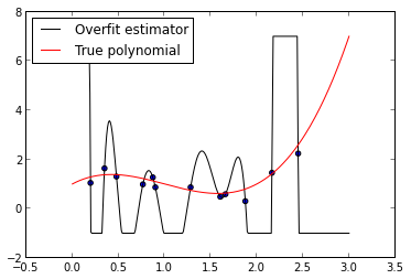
As we can see from this plot, the fitted \(N - 1\)-degree polynomial is significantly less smooth than the true polynomial, \(p\). This roughness results from the fact that the \(N - 1\)-degree polynomial has enough parameters to account for the noise in the model, instead of the true underlying structure of the data. Such a model is called overparametrized or overfit. While its mean squared error on the training data, its in-sample error, is quite small,

mean_squared_error(overfit_model.predict(xs), ys)

2.0039043409236146e-15

It will not, however, perform well when used to predict the value of \(p\) at points not in the training set. (Note that this in-sample error should theoretically be zero. The small positive value is due to rounding errors.) To illustrate this inaccuracy, we generate ten more points uniformly distributed in the interval \([0, 3]\) and use the overfit model to predict the value of \(p\) at those points.

N_prediction = 10

prediction_xs = stats.uniform.rvs(left, right, size=N_prediction)
prediction_eps = stats.norm.rvs(0, np.sqrt(var), size=N_prediction)
prediction_ys = p(prediction_xs) + prediction_eps

mean_squared_error(overfit_model.predict(prediction_xs), prediction_ys)

19.539402955310337

We see that the prediction error is many orders of magnitude larger than the in- sample error. This awful predictive performance of a model with excellent in- sample error illustrates the need for cross-validation to prevent overfitting.

Here we use scikit-learn’s GridSearchCV to choose the degree of the polynomial using three-fold cross-validation. We constrain our search to degrees between one and twenty-five.

estimator = PolynomialRegression()
degrees = np.arange(1, 25)
cv_model = GridSearchCV(estimator,
                        param_grid={'deg': degrees},
                        scoring='mean_squared_error')
cv_model.fit(xs, ys);

cv_model.best_params_, cv_model.best_estimator_.coef_

({'deg': 3}, array([ 1.03303734, -3.21335403,  2.26034212,  0.88016067]))

We see that cross-validation has chosen the correct degree of the polynomial, and recovered the same coefficients as the model with known degree.

fig = plt.figure()
ax = fig.add_subplot(111)

plt.scatter(xs, ys);
ax.plot(plot_xs, np.clip(overfit_model.predict(plot_xs), -1, 7), color='k', label='Overfit estimator');
plt.plot(plot_xs, cv_model.predict(plot_xs), color='b', label='Cross-validated estimator');
ax.plot(plot_xs, p(plot_xs), color='r', label='True polynomial');
ax.legend(loc=2);

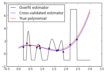
We see that the cross-validated estimator is much smoother and closer to the true polynomial than the overfit estimator. The in-sample error of the cross- validated estimator is

mean_squared_error(cv_model.predict(xs), ys)

0.039089250360265018

and the prediction error is

mean_squared_error(cv_model.predict(prediction_xs), prediction_ys)

0.15873290784021762

These errors are much closer than the corresponding errors of the overfit model.

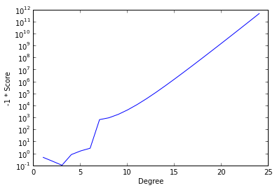
To further illustrate the advantages of cross-validation, we show the following graph of the negative score versus the degree of the fit polynomial.

fig = plt.figure()
ax = fig.add_subplot(111)

scores = np.array([grid_score.mean_validation_score for grid_score in cv_model.grid_scores_])
ax.plot(degrees, -scores);
ax.set_yscale('log');
ax.set_ylabel('-1 * Score');
ax.set_xlabel('Degree');

The cross-validation process seeks to maximize score and therefore minimize the negative score. (We have plotted negative score here in order to be able to use a logarithmic scale.) We see that this quantity is minimized at degree three and explodes as the degree of the polynomial increases (note the logarithmic scale). While overfitting the model may decrease the in-sample error, this graph shows that the cross-validation score and therefore the predictive accuracy increases at a phenomenal rate.

This post is available as an IPython notebook here.

Discussion on Hacker News