Nonparametric Bayesian Regression with Gaussian Processes
Nonparametric statistics is a branch of statistics concerned with analyzing data without assuming that the data are generated from any particular probability distribution. Since they make fewer assumptions about the process that generated the data, nonparametric tests are often more generally applicable than their parametric counterparts. Nonparametric methods are also generally more robust than their parametric counterparts. These advantages are balanced by the fact that when the data are generated by a known probability distribution, the appropriate parametric tests are more powerful.
In this post, we’ll explore a Bayesian approach to nonparametric regression, which allows us to model complex functions with relatively weak assumptions.
A Prior on Functions
We will study the model \(y = f(x) + \varepsilon\), where \(f\) is the true regression function we wish to model, and \(\varepsilon\) is Gaussian noise. Given observations \((x_1, y_1), \ldots, (x_n, y_n)\) from this model, we wish to predict the value of \(f\) at new \(x\)-values. Let \(X = (x_1, \ldots, x_n)^\top\) be the column vector of the observed \(x\)-values, and similarly let \(Y = (y_1, \ldots, y_n)^\top\). Our goal is to use these observations to predict the value of \(f\) at any given point with as much accuracy as possible.
The Bayesian approach to this problem is to calculate the posterior predictive distribution, \(p(f_* | X, Y, x_*)\) of the value of \(f\) at a point \(x_*\). With this distribution in hand, we, if necessary, employ decision-theoretic machinery to produce point estimates for the value of \(f\) at \(x_*\).
As the nonparametric approach makes as few assumptions about the regression function as possible, a natural first step would seem to be to place a prior distribution \(\pi(f)\) on all possible regression functions. In this case, the posterior predictive distribution is
\[\begin{align*} p(f_* | X, Y, x_*) & = \int_f p(f_* | f, x_*)\ p(f | X, Y)\ df \\ & \propto \int_f p(f_* | f, x_*)\ p(Y | f, X)\ \pi(f) df. \end{align*}\]
Observant readers have certainly noticed that above we integrate with respect to an unspecified measure \(df\). If we make the often-reasonable assumption that \(f\) is continuous on a compact interval \([0, T]\) (for \(T < \infty\)), we may choose \(df\) to be the Weiner measure, which is closely related to Brownian motion. Unfortunately, this approach has a few drawbacks. First, it may be difficult to choose a decent prior on the contiuous functions on the interval \([0, T]\) (even the uniform prior will be improper). Even if we manage to choose a good prior, the integral with respect to the Weiner measure may not be easy (or even possible) to calculate or approximate.
Gaussian Processes
The key realization about this situation that allows us to sidestep the difficulty in calculating the posterior predictive distribution in the manner detailed above is to consider the joint distribution of the observed and predicted values of \(f\). Suppose that given our observations, we want to predict the value of \(f\) at the points \(x_{*, 1}, \ldots x_{*, m}\). Again, let \(X_* = (x_{*, 1}, \ldots, x_{*, m})^\top\) and \(Y_* = (f(x_{*, 1}), \ldots, f(x_{*, m}))^\top\). With this notation, we want to model the joint distribution of the random variables \(Y\) and \(Y_*\). After choosing a joint distribution, we can condition on the observed value of \(Y\) (and \(X\) and \(X_*\)) to obtain a posterior predictive distribution for \(Y_*\). In this approach, specifying the joint distribution of \(Y\) and \(Y_*\) has taken the place of specifying a prior distribution on regression functions.
We obtain a flexible model for the joint distribution of \(Y\) and \(Y_*\) by considering the set \(\{f(x) | x \in \mathbb{R}\}\) to be a Gaussian Process. That is, for any finite number of points \(x_1, \ldots, x_n \in \mathbb{R}\), the random variables \(f(x_1), \ldots, f(x_n)\) have a multivariate normal distribution. While at first it may seem that modelling \(f\) with a Gaussian process is a parametric approach to the problem, mean vector and covarience matrix of the multivariate normal (generally) depend explicitly on the points \(x_1, \ldots, x_n\), making this approach quite flexible and nonparametric. The Gaussian process for \(f\) is specified by a mean function \(m(x)\) and a covariance function \(k(x, x')\). In this context, we write that \(f \sim GP(m, k)\). The advantage of this approach is that the Gaussian process model is quite flexible, due to the ability to specify different mean and covariance functions, while still allowing for exact calculation of the predictions.
For the purposes of this post, we will assume that the mean of our Gaussian process is zero; we will see later that this is not a terribly restrictive assumption. Much more important than the choice of a mean function is the choice of a covariance function, \(k\). In general, \(k\) must be positive-definite in the sense that for any \(X = (x_1, \ldots x_n)\), \(k(X, X) = (k(x_i, x_j))_{i, j}\) is a positive-definite matrix. This restriction is necessary in order for the covariance matrices of the multivariate normal distributions obtained from the Gaussian process to be sensible. There are far too many choices of covariance function to list in detail here. In this post, we will use the common squared-exponential covariance function,
\[k(x, x') = \exp\left(-\frac{(x - x')^2}{2 \ell^2}\right).\]
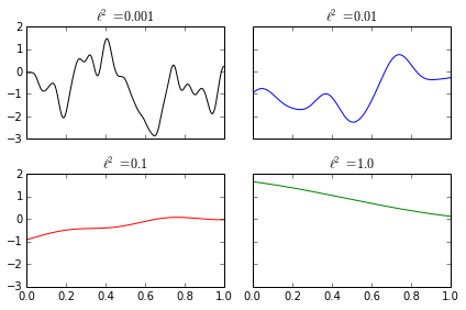
The parameter \(\ell\) controls how quickly the function \(f\) may fluctuate. Small values of \(\ell\) allow \(f\) to fluctuate rapidly, while large values of \(\ell\) allow \(f\) to fluctuate slowly. The following diagram shows samples from Gaussian processes with different values of \(\ell\).
def k(x1, x2, l=1.0):
    return np.exp(-np.subtract.outer(x1, x2)**2 / (2 * l**2))

def sample_gp(xs, m=None, k=k, l=1.0, size=1):
    if m is None:
        mean = np.zeros_like(xs)
    else:
        mean = m(xs)

    cov = k(xs, xs, l)

    samples = np.random.multivariate_normal(mean, cov, size=size)

    if size == 1:
        return samples[0]
    else:
        return samples
Gaussian Process Regression
Now that we have introducted the basics of Gaussian processes, it is time to use them for regression. Using the notation from above, the joint distribution of \(Y\), the values of \(f\) at the observed points, and \(Y_*\), the values of \(f\) at the points to be predicted, is normal with mean zero and covariance matrix
\[\Sigma = \begin{pmatrix} k(X, X) + \sigma^2 I & k(X, X_*) \\ k(X_*, X) & k(X_*, X_*) \end{pmatrix}.\]
In \(\Sigma\), only the top left block contains a noise term. The top right and bottom left blocks have no noise term because the entries of \(Y\) and \(Y_*\) are uncorrelated (since the noise is i.i.d). The bottom right block has no noise term because we want to predict the actual value of \(f\) at each point \(x_*, i\), not its value plus noise.
Conditioning on the observations \(Y = y\), we get that \(Y_* | Y = y\) is normal with mean \(\mu_y = k(X_*, X) (k(X, X) + \sigma^2 I)^{-1} y\) and covariance \(\Sigma_y = k(X_*, X_*) - k(X_*, X) (k(X, X) + \sigma^2 I)^{-1} k(X, X_*)\).
A Toy Example
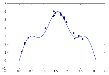
As a toy example, we will use Gaussian process regression to model the function \(f(x) = 5 \sin x + \sin 5 x\) on the interval \([0, \pi]\), with i.i.d. Gaussian noise with standard deviation \(\sigma = 0.2\) using twenty samples.
def f(x):
    return 5 * np.sin(x) + np.sin(5 * x)


n = 20
sigma = 0.2

sample_xs = sp.stats.uniform.rvs(scale=np.pi, size=n)
sample_ys = f(sample_xs) + sp.stats.norm.rvs(scale=sigma, size=n)

xs = np.linspace(0, np.pi, 100)
The following class implements this approach to Gaussian process regression as a sublcass of scikit-learn’s sklearn.base.BaseEstimator.
class GPRegression(BaseEstimator):
    def __init__(self, l=1.0, sigma=0.0):
        self.l = l
        self.sigma = sigma

    def confidence_band(self, X, alpha=0.05):
        """
        Calculates pointwise confidence bands with coverage 1 - alpha
        """
        mean = self.mean(X)
        cov = self.cov(X)
        std = np.sqrt(np.diag(cov))

        upper = mean + std * sp.stats.norm.isf(alpha / 2)
        lower = mean - std * sp.stats.norm.isf(alpha / 2)

        return lower, upper

    def cov(self, X):
        return k(X, X, self.l) - np.dot(k(X, self.X, self.l),
                                 np.dot(np.linalg.inv(k(self.X, self.X, self.l)
                                                      + self.sigma**2 * np.eye(self.X.size)),
                                        k(self.X, X, self.l)))

    def fit(self, X, y):
        self.X = X
        self.y = y

    def mean(self, X):
        return np.dot(k(X, self.X, self.l),
               np.dot(np.linalg.inv(k(self.X, self.X, self.l)
                        + self.sigma**2 * np.eye(self.X.size)),
                      self.y))

    def predict(self, X):
        return self.mean(X)
Subclassing BaseEstimator allows us to use scikit-learn’s cross-validation tools to choose the values of the hyperparameters \(\ell\) and \(\sigma\).
gp = GPRegression()
param_grid = {
              'l': np.linspace(0.01, 0.6, 50),
              'sigma': np.linspace(0, 0.5, 50)
              }

cv = GridSearchCV(gp, param_grid, scoring='mean_squared_error')
cv.fit(sample_xs, sample_ys);
Cross-validation yields the following parameters, which produce a relatively small mean squared error.
model = GPRegression(**cv.best_params_)
model.fit(sample_xs, sample_ys)
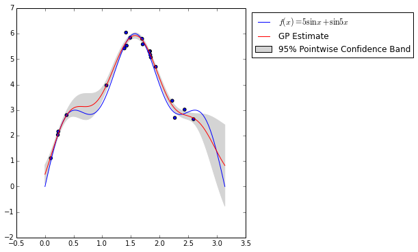
cv.best_params_{'l': 0.40734693877551015, 'sigma': 0.1020408163265306}The figure below shows the true regression function, \(f(x) = 5 \sin x + \sin 5 x\) along with our Gaussian process regression estimate. It also shows a 95% pointwise confidence band around the estimated regression function.

Note now near observed points, the confidence band shrinks drastically, while away from observed points it expands rapidly.
Properties of Gaussian Process Regression
As our toy example shows, Gaussian processes are powerful and flexible tools for regression. Although we have only just scratched the surface of this vast field, some remarks about the general properties and utility of Gaussian process regression are in order. For a much more extensive introduction to Gaussian process consult the excellent book Gaussian Processes for Machine Learning, which is freely available online.
In general, Gaussian process regression is only effective when the covariance function and its parameters are appropriately chosen. Although we have used cross-validation to choose the parameter values in our toy example, for more serious problems, it is often much quicker to maximize the marginal likelihood directly by calculating its gradient.
Our implementation of Gaussian process regression is numerically unstable, as it directly inverts the matrix \(k(X, X) + \sigma^2 I\). A more stable approach is to calculate the Cholesky decomposition of this matrix. Unfortuantely, calculating the Cholesky decomposition of an \(n\)-dimensional matrix takes \(O(n^3)\) time. In the context of Gaussian process regression, \(n\) is the number of observations. If the number of training points is significant, the cubic complexity may be prohibitive. A number of approaches have been developed to approximate the results of Gaussian process regression with larger training sets. For more details on these approximations, consult Chapter 8 of Gaussian Processes for Machine Learning.
This post is available as an IPython notebook.