A Bayesian Alternative to Synthetic Control Comparative Case Studies in Python with PyMC3
Recently I had cause to be perusing Yiqing Xu’s research and dove deep into the 2020 paper A Bayesian Alternative to Synthetic Control for Comparative Case Studies1 (BASC-CCS from now on). In an effort to better understand the method introduced in this paper, I decided to replicate (most of) the results form the simulation study described in Sections 4.1 and A.4.1 in Python using PyMC3.
BASC-CCS uses time series cross sectional data (TSCS) to infer causal effects from observational data where direct control of the treatment mechanism is not possible. As such it falls under the umbrella of causal inference methods. More specifically, it uses the Bayesian approach that treats causal inference from observational data as a problem of imputing missing (control) data for treated units.
Generate the Data
We begin by generating the data to be modeled. First we make the necessary Python imports and do some light housekeeping.
%matplotlib inlinefrom warnings import filterwarningsfrom aesara import tensor as at
import arviz as az
import matplotlib as mpl
from matplotlib import pyplot as plt
from matplotlib.lines import Line2D
import numpy as np
import pymc3 as pm
import scipy as sp
import seaborn as sns
import xarray as xrYou are running the v4 development version of PyMC3 which currently still lacks key features. You probably want to use the stable v3 instead which you can either install via conda or find on the v3 GitHub branch: https://github.com/pymc-devs/pymc3/tree/v3filterwarnings('ignore', category=pm.ImputationWarning, module='pymc3')mpl.rcParams['figure.figsize'] = (8, 6)
sns.set(color_codes=True)BASC-CCS is designed for TSCS where a number of units are observed over a period of time. Following the BASC-CCS paper, we simulate data from \(N = 50\) units over \(T = 30\) time periods.
N = 50
T = 30

t = np.arange(T)
In this simulation 10% of the units will be treated starting at time \(T_{\mathrm{treat}} = 21\).
T_treat = 21
P_treat = 0.1
Which units are treated will be determined by a linear combination of two unobserved latent factors, drawn from a standard normal distribution for each unit, \(\Gamma_{i, 1}, \Gamma_{i, 2} \sim N(0, 1)\) (note that we use capital letters for simulated quantities and the corresponding lowercase letters for the corresponding inferred parameters).
SEED = 12345 # for reproducibility

rng = np.random.default_rng(SEED)
Γ = rng.normal(size=(N, 2))Treatment is determined according to the variable
\[\mathrm{tr}_i = 0.7 \cdot \Gamma_{i, 1} + 0.3 \cdot \Gamma_{i, 2} + \varepsilon^{\Gamma}_i,\]
where \(\varepsilon^{\Gamma}_i \sim N(0, 0.25).\)
tr = Γ.dot([0.7, 0.3]) + rng.normal(0., 0.5, size=N)The five units with the largest values of \(tr_i\) are treated.
treat_crit = np.percentile(tr, 100 * (1. - P_treat))
treated = tr > treat_crit
n_treated = treated.sum()
n_treated5The following plot shows the relationship between the latent values \(\Gamma_i\) and which units are treated.
CMAP = 'winter'fig, ax = plt.subplots(figsize=(8, 8))
ax.set_aspect('equal');
norm = plt.Normalize(tr.min(), tr.max())
sns.scatterplot(x=Γ[~treated, 0], y=Γ[~treated, 1], hue=tr[~treated],
hue_norm=norm, palette=CMAP,
label="Untreated", legend=False,
ax=ax);
sns.scatterplot(x=Γ[treated, 0], y=Γ[treated, 1], hue=tr[treated],
s=100, marker='s',
hue_norm=norm, palette=CMAP,
label="Treated", legend=False,
ax=ax);
Γ_mult = 1.05
Γ_min, Γ_max = Γ_mult * Γ.min(), Γ_mult * Γ.max()
plot_Γ = np.linspace(Γ_min, Γ_max, 100)
ax.plot(plot_Γ, (treat_crit - 0.7 * plot_Γ) / 0.3,
c='k', ls='--', label="Treatment threshold\n(noiseless)");
sm = plt.cm.ScalarMappable(norm=norm, cmap=CMAP)
cbar = fig.colorbar(sm)
ax.set_xlim(Γ_min, Γ_max);
ax.set_xlabel(r"$\Gamma_{i, 1}$");
ax.set_ylim(Γ_min, Γ_max);
ax.set_ylabel(r"$\Gamma_{i, 2}$");
cbar.set_label(r"$\mathrm{tr}_i$");
ax.legend(loc='upper left');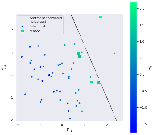
The inclusion of the noise term \(\varepsilon^{\Gamma}_i\) causes some of the treated units to be below the treatment threshold line in this plot and some of the points above the treatment threshold line to not be treated.
We now generate \(K = 10\) covariates for each unit, one of which is a constant intercept and the rest of which follow a standard normal distribution.
K = 10X = np.empty((N, K))
X[:, 0] = 1.
X[:, 1:] = rng.normal(size=(N, K - 1))Following the paper, the first \(K_* = 4\) covariates influence the outcome, and the rest are uncorrelated with it. The true regression coefficients, \(B_j\) are taken from the BASC-CCS paper.
K_star = 4B = np.zeros(K)
B[:K_star] = 3., 6., 4., 2.The influence of each of the first \(K_*\) covariates varies by unit, according to \(A_{i, j} \sim N\left(0, \left(\frac{B_j}{2}\right)^2\right)\).
A = np.zeros((N, K))
A[:, :K_star] = rng.normal(0., 0.5 * B[:K_star], size=(N, K_star))
The influence of these first \(K_*\) covariates also varies over time according to an \(AR(1)\) process \(\Xi_{j, t}\) with autocorrelation of \(0.6\) and standard normal innovations.
def ar1(k, innov):
    t = np.arange(innov.shape[-1])
    expon = sp.linalg.toeplitz(t)

    return np.dot(innov, np.triu(np.power(k, expon)))
innov_Ξ = rng.normal(size=(K_star, T))
Ξ = np.zeros((K, T))
Ξ[:K_star] = ar1(0.6, innov_Ξ)fig, ax = plt.subplots(figsize=(8, 6))
ax.plot(t, Ξ.T, c='k', alpha=0.75);
ax.set_xlabel("$t$");
ax.set_ylabel(r"$\Xi_{i, t}$");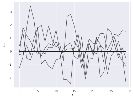
The horizontal lines at zero here correspond to the \(K - K_*\) covariates that have no influence on the outcome and do not vary over time.
The noise in outcomes is related to the latent parameters \(\Gamma_i\) through factor loadings \(F_t\), which also follow an \(AR(1)\) process with autocorrelation of \(0.7\) and standard normal innovations.
innov_F = rng.normal(size=(2, T))

F = ar1(0.7, innov_F)
fig, ax = plt.subplots(figsize=(8, 6))
ax.plot(t, F.T, c='k', alpha=0.75);
ax.set_xlabel("$t$");
ax.set_ylabel(r"$F_{i, t}$");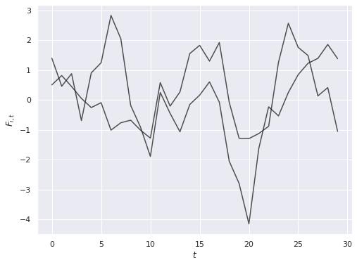
Finally, we simulate the treament effects, which are
\[ \Delta_{i, t} = \begin{cases} t - T_{\mathrm{treat}} + \varepsilon^{\mathrm{treat}}_{i, t} & \mathrm{if}\ t > T_{\mathrm{treat}} \\ 0 & \mathrm{if}\ t \leq T_{\mathrm{treat}} \end{cases} \]
where \(\varepsilon^{\mathrm{treat}}_{i, t} \sim N(0, 0.25)\).
Δ = np.zeros((N, T))
Δ[:, T_treat:] = t[T_treat:] - T_treat \
                    + rng.normal(0., 0.5, size=(N, T - T_treat))
The array w indicates which units where treated at a given time, with
\[ w_{i, t} = \begin{cases} 1 & \mathrm{if\ unit}\ i\ \mathrm{is\ treated\ at\ time}\ t \\ 0 & \mathrm{otherwise} \end{cases}. \]
w = np.zeros((N, T))
w[treated, T_treat:] = 1
We plot the treatment effects that our model will attempt to recover.
fig, ax = plt.subplots(figsize=(8, 6))

ax.plot(t, (Δ * w)[~treated][0],
        c='k', label="Untreated");
ax.plot(t, (Δ * w)[treated][0],
        c='r', alpha=0.75,
        label="Treated");
ax.plot(t, (Δ * w)[treated][1:].T,
        c='r', alpha=0.75);

ax.set_xlabel("$t$");
ax.set_ylabel(r"$\Delta_{i, t} \cdot w_{i, t}$");
ax.legend(loc='upper left');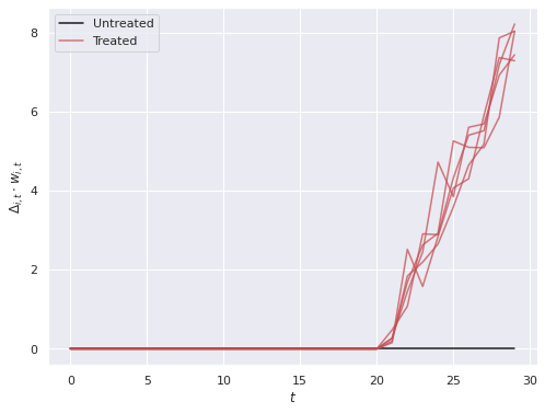
We combine each of these components to generate the data to be modeled.
Θ = (B + A)[..., np.newaxis] + Ξ[np.newaxis]
XΘ = (X[..., np.newaxis] * Θ).sum(axis=1)
We combine the reatment effects, the effects of the covariates, the effects of the latent factors, and standard normal noise to get the observed outcomes, \(y_{i, t}\).
y = Δ * w + XΘ + Γ.dot(F) + rng.normal(size=(N, T))fig, ax = plt.subplots(figsize=(8, 6))
ax.axvline(T_treat, c='k', ls='--',
label="$T_{\mathrm{treat}}$");
ax.plot(t, y[~treated].T, c='k', alpha=0.5);
ax.plot([], [], c='k', alpha=0.5,
label="Untreated");
ax.plot(t, y[treated].T, c='r', lw=3, alpha=0.75);
ax.plot([], [], c='r', alpha=0.75,
label="Treated");
ax.set_xlabel("$t$");
ax.set_ylabel("$y_{i, t}$");
ax.legend(loc="upper left");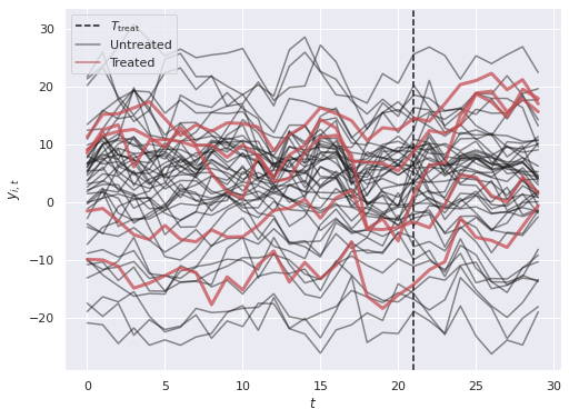
We see that the treated units have outcomes that generally trend up after \(T_{\mathrm{treat}}\), but there is a lot of visual noise to interpret when comparing those to the untreated units. Thee BASC-CCS model w will build in the next section will help to quantify the difference and cut through this noise.
Modeling
Unidentified latent factors
We begin with a model that has unidentified latent factors in order to determine which factors we should constrain to best identify our model. For more details about implementing factor analysis models in PyMC see my previous post on the topic.
Since we are using the Bayesian causal-inference-as-missing-data paradigm, we define the control observations as a masked array, with entries masked when \(w_{i, t} = 1\), indicating that the \(i\)-th unit was treated at time \(t\).
y_ctrl = np.ma.array(y, mask=w)For simplicity our model will use two latent factors, even though in general we do not know the true number of latent factors. For a more rigorous discussion of how to choose the number of latent factors, see Machine Learning, A Probabilistic Perspective2, §12.3.
N_factor = 2We define the coordinates for our parameters. (For more information on how to get PyMC3 to interact nicely with xarray via coordinates, see Oriol Abril’s excellent post on the subject.)
coords = {
    "unit": np.arange(N),                        # units
    "fact": np.arange(N_factor),                 # latent factors
    "feat": np.arange(K),                        # features
    "time": t,                                   # time
    "time_block": np.arange(T - (N_factor + 1))  # block of time for identifying factors
}
We put centered normal priors on our shared regression coefficients, \(\beta_j\). This prior differs from the one in the paper, which uses a sparse prior for these coefficients. Fortunately since we are using a modular probabilistic programming library, this prior can be changed relatively easily.
with pm.Model(coords=coords) as ref_model:
    β = pm.Normal("β", 0., 5., dims="feat")
We put hierarchical normally distributed priors with mean zero (for identifiability) on the per-unit random effects \(\alpha_{i, j}\) and the per-time random effects \(\xi_{j, t}\).
# the scale necessary to make a halfnormal distribution
# have unit variance
HALFNORMAL_SCALE = 1. / np.sqrt(1. - 2. / np.pi)

def noncentered_normal(name, dims, μ=None,):
    if μ is None:
        μ = pm.Normal(f"μ_{name}", 0., 5.)

    Δ = pm.Normal(f"Δ_{name}", 0., 1., dims=dims)
    σ = pm.HalfNormal(f"σ_{name}", 5. * HALFNORMAL_SCALE)

    return pm.Deterministic(name, μ + Δ * σ)
with ref_model:
α = noncentered_normal("α", ("unit", "feat"), μ=0.)
ξ = noncentered_normal("ξ", ("feat", "time"), μ=0.)Note that here we do not use the fact that the true values of \(\Xi_{j, t}\) form an AR(1) process.
We combine \(\beta_j\), \(\alpha_{i, j}\), and \(\xi_{j, t}\) to form the full coefficient cube, \(\theta_{i, j, t}\).
θ = β[np.newaxis, :, np.newaxis] \
        + α[..., np.newaxis] \
        + ξ[np.newaxis, ...]
We build latent factor component of the model as in the previous post, knowing that this model specificiation is only identified up to reflections of f_unid and γ_unid.
with ref_model:
    f_pos_row = pm.HalfNormal("f_pos_row", HALFNORMAL_SCALE,
                              dims="fact")
    f_block_unid = pm.Normal("f_block_unid", 0., 1.,
                             dims=("time_block", "fact"))
    f_unid = at.concatenate((
        at.eye(N_factor),
        at.shape_padleft(f_pos_row),
        f_block_unid
    ))
    γ_unid = pm.Normal("γ_unid", 0., 1., dims=("unit", "fact"))
Finally, we specify our observational likelihood.
with ref_model:
    μ_ctrl = (X[..., np.newaxis] * θ).sum(axis=1) + γ_unid.dot(f_unid.T)

    σ = pm.HalfNormal("σ", 5. * HALFNORMAL_SCALE)
    obs_ctrl = pm.Normal("obs_ctrl", μ_ctrl, σ, observed=y_ctrl)
We now draw 100 samples from this unidentified model.
CORES = 3

SAMPLE_KWARGS = {
    "cores": CORES,
    "random_seed": [SEED + i for i in range(CORES)],
    "return_inferencedata": True
}
with ref_model:
ref_trace = pm.sample(tune=100, draws=100, **SAMPLE_KWARGS)Only 100 samples in chain.
Auto-assigning NUTS sampler...
Initializing NUTS using jitter+adapt_diag...
Multiprocess sampling (3 chains in 3 jobs)
NUTS: [β, Δ_α, σ_α, Δ_ξ, σ_ξ, f_pos_row, f_block_unid, γ_unid, σ, obs_ctrl_missing]100.00% [600/600 02:14<00:00 Sampling 3 chains, 18 divergences]
Sampling 3 chains for 100 tune and 100 draw iterations (300 + 300 draws total) took 136 seconds.
There were 18 divergences after tuning. Increase `target_accept` or reparameterize.
The acceptance probability does not match the target. It is 1.0, but should be close to 0.8. Try to increase the number of tuning steps.
The rhat statistic is larger than 1.4 for some parameters. The sampler did not converge.
The number of effective samples is smaller than 10% for some parameters.az.rhat(ref_trace).max()<xarray.Dataset>
Dimensions: ()
Data variables:
β float64 1.813
Δ_α float64 1.885
σ_α float64 1.814
Δ_ξ float64 1.86
σ_ξ float64 1.805
f_pos_row float64 1.727
f_block_unid float64 1.818
γ_unid float64 1.808
σ float64 1.832
obs_ctrl_missing float64 1.82
α float64 1.85
ξ float64 1.848
-
-
-
-
β()float641.813
array(1.81270912)
-
Δ_α()float641.885
array(1.88526959)
-
σ_α()float641.814
array(1.81400238)
-
Δ_ξ()float641.86
array(1.85974353)
-
σ_ξ()float641.805
array(1.80451891)
-
f_pos_row()float641.727
array(1.72748944)
-
f_block_unid()float641.818
array(1.81831663)
-
γ_unid()float641.808
array(1.80812046)
-
σ()float641.832
array(1.83187637)
-
obs_ctrl_missing()float641.82
array(1.81951939)
-
α()float641.85
array(1.84973862)
-
ξ()float641.848
array(1.84825114)
-
-
As expected, the \(\hat{R}\) parameters are quite high, indiciating that the chains have not converged well. This behavior is expected, since we know that this model is reflection-invariant and therefore has a multimodal posterior.
As in the previous post on identification in factor analysis, we choose a row of f_block_unid that we constrain to have all positive entries and change the signs of the entries f_block_unid and γ_unid so that they have the same relationship with the signs of this row. We choose the row that has the chain whose latent factors have the largest posterior expected distance from the origin.
block_mean = (ref_trace.posterior["f_block_unid"]
                       .mean(dim="draw"))
block_mean_norm = np.square(block_mean).sum(dim="fact")
sign_row = (block_mean_norm.max(dim="chain")
                           .argmax()
                           .item())
sign_chain = (block_mean_norm.sel({"time_block": sign_row})
                             .argmax()
                             .item())
target_sign = (np.sign(block_mean.sel({"chain": sign_chain,
"time_block": sign_row}))
.data)We can now specify the identified model, which is largely the same as the previous model.
with pm.Model(coords=coords) as model:
    β = pm.Normal("β", 0., 5., dims="feat")
    α = noncentered_normal("α", ("unit", "feat"), μ=0.)
    ξ = noncentered_normal("ξ", ("feat", "time"), μ=0.)
    θ = β[np.newaxis, :, np.newaxis] \
            + α[..., np.newaxis] \
            + ξ[np.newaxis, ...]

    f_pos_row = pm.HalfNormal("f_pos_row", HALFNORMAL_SCALE,
                              dims="fact")
    f_block_unid = pm.Normal("f_block_unid", 0., 1.,
                             dims=("time_block", "fact"))

    γ_unid = pm.Normal("γ_unid", 0., 1., dims=("unit", "fact"))
We now enforce the sign constraints that will break the reflectional invariance of the previous model and specify the observational likelihood.
with model:
    unid_sign = at.sgn(f_block_unid[sign_row])

    f_block = pm.Deterministic(
        "f_block", target_sign * unid_sign * f_block_unid,
        dims=("time_block", "fact")
    )
    f = at.concatenate((
        at.eye(N_factor),
        at.shape_padleft(f_pos_row),
        f_block
    ))

    γ = pm.Deterministic(
        "γ", target_sign * unid_sign * γ_unid,
        dims=("unit", "fact")
    )

    μ_ctrl = (X[..., np.newaxis] * θ).sum(axis=1) + γ.dot(f.T)

    σ = pm.HalfNormal("σ", 5. * HALFNORMAL_SCALE)
    obs_ctrl = pm.Normal("obs_ctrl", μ_ctrl, σ, observed=y_ctrl)
We now sample from this identified model.
with model:
    trace = pm.sample(**SAMPLE_KWARGS)
Auto-assigning NUTS sampler...
Initializing NUTS using jitter+adapt_diag...
Multiprocess sampling (3 chains in 3 jobs)
NUTS: [β, Δ_α, σ_α, Δ_ξ, σ_ξ, f_pos_row, f_block_unid, γ_unid, σ, obs_ctrl_missing]100.00% [6000/6000 13:54<00:00 Sampling 3 chains, 0 divergences]
Sampling 3 chains for 1_000 tune and 1_000 draw iterations (3_000 + 3_000 draws total) took 835 seconds.
The rhat statistic is larger than 1.4 for some parameters. The sampler did not converge.
The estimated number of effective samples is smaller than 200 for some parameters.
For the moment we ignore the convergence warnings, because we expect the \(\hat{R}\) values for f_block_unid and γ_unid to be high.
The energy plot shows no cause for concern.
az.plot_energy(trace);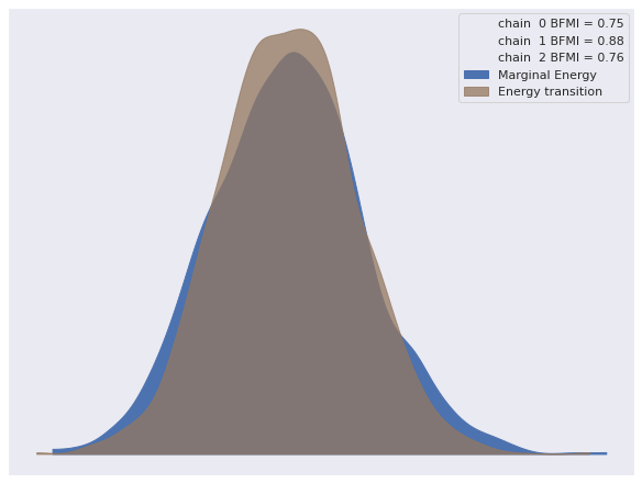
Ignoring the variables we know are not identified, all of our \(\hat{R}\) statistics are reasonable as well.
rhat_var_names = [
    var_name for var_name in trace.posterior.data_vars
        if not var_name.endswith("_unid")
]
az.rhat(trace, var_names=rhat_var_names).max()<xarray.Dataset>
Dimensions: ()
Data variables:
β float64 1.004
Δ_α float64 1.007
σ_α float64 1.003
Δ_ξ float64 1.008
σ_ξ float64 1.0
f_pos_row float64 1.002
σ float64 1.002
obs_ctrl_missing float64 1.004
α float64 1.008
ξ float64 1.008
f_block float64 1.008
γ float64 1.008
-
-
-
-
β()float641.004
array(1.00389839)
-
Δ_α()float641.007
array(1.00650723)
-
σ_α()float641.003
array(1.00252306)
-
Δ_ξ()float641.008
array(1.00802131)
-
σ_ξ()float641.0
array(1.00025354)
-
f_pos_row()float641.002
array(1.00226488)
-
σ()float641.002
array(1.00224675)
-
obs_ctrl_missing()float641.004
array(1.00359828)
-
α()float641.008
array(1.00811494)
-
ξ()float641.008
array(1.00801751)
-
f_block()float641.008
array(1.00819455)
-
γ()float641.008
array(1.00805011)
-
-
The model has recovered the true regression coefficients reasonably well.
ax, = az.plot_forest(trace, var_names=["β"],
                     combined=True, hdi_prob=0.95)

ax.scatter(B[::-1], ax.get_yticks(),
           c='k', zorder=5, label="Actual");

ax.set_yticklabels([]);
ax.set_ylabel(r"$\beta_j$");

ax.legend(loc='upper left');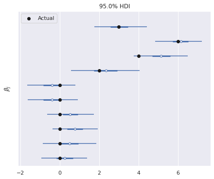
We now turn to estimating the causal effect. First we build an array of the posterior imputed control outcomes for the treated units.
post_treat_ctrl = xr.DataArray(
    trace.posterior["obs_ctrl_missing"]
          .data
          .reshape((CORES, 1000, n_treated, T - T_treat)),
    dims=(
        "chain", "draw",
        "treat_unit", "treat_time"
    )
)post_treat_ctrl.head()<xarray.DataArray (chain: 3, draw: 5, treat_unit: 5, treat_time: 5)>
array([[[[ 1.25759892e+01,  1.30612264e+01,  1.57087369e+01,
           1.49536257e+01,  1.64677110e+01],
         [-4.12810485e-02,  6.26047750e+00,  7.79874263e+00,
           1.23859034e+01,  1.61490831e+01],
         [ 7.27955473e+00,  1.04034349e+01,  1.12521199e+01,
           1.11063292e+01,  1.13530200e+01],
         [-5.36650155e+00, -5.83322477e+00, -3.35144524e+00,
           3.44000735e+00,  1.88207349e+00],
         [-1.31260800e+01, -1.22691019e+01, -1.33695535e+01,
          -5.94977044e+00, -8.61557509e+00]],

        [[ 1.30278045e+01,  1.42052058e+01,  1.40630688e+01,
           1.47218969e+01,  1.93233792e+01],
         [ 2.45746861e+00,  3.67240422e+00,  6.87289651e+00,
           8.61550996e+00,  1.48857372e+01],
         [ 8.68996670e+00,  1.22336995e+01,  1.01608424e+01,
           9.78275733e+00,  1.42336802e+01],
         [-6.32208820e+00, -3.22852886e+00, -1.89722169e+00,
           3.30217994e-01,  3.78225547e+00],
         [-1.53244972e+01, -1.35265466e+01, -1.36205170e+01,
...
           1.35873648e+01,  1.50553915e+01],
         [ 3.01241871e+00,  5.42217922e+00,  6.50204080e+00,
           1.15586759e+01,  1.33643026e+01],
         [ 7.65560768e+00,  1.29871011e+01,  9.75434111e+00,
           1.09479191e+01,  1.26587440e+01],
         [-3.59855020e+00, -4.76761066e+00, -4.10285725e+00,
           2.14369279e+00,  3.28661610e-01],
         [-1.39193859e+01, -1.79066255e+01, -1.26329862e+01,
          -4.73557646e+00, -7.94774028e+00]],

        [[ 1.38132791e+01,  1.24831973e+01,  1.20970456e+01,
           1.37274249e+01,  1.51289416e+01],
         [ 3.95173624e+00,  5.69156061e+00,  6.21128104e+00,
           1.20260114e+01,  1.34918240e+01],
         [ 7.22084256e+00,  1.30855164e+01,  9.73445859e+00,
           1.10445040e+01,  1.27090074e+01],
         [-3.85094179e+00, -3.93828746e+00, -3.88376440e+00,
           1.53955903e+00,  8.58625045e-01],
         [-1.39993793e+01, -1.79798655e+01, -1.25980525e+01,
          -4.70834640e+00, -7.87338772e+00]]]])
Dimensions without coordinates: chain, draw, treat_unit, treat_time
- chain: 3
- draw: 5
- treat_unit: 5
- treat_time: 5
-
12.58 13.06 15.71 14.95 16.47 … -14.0 -17.98 -12.6 -4.708 -7.873
array([[[[ 1.25759892e+01, 1.30612264e+01, 1.57087369e+01, 1.49536257e+01, 1.64677110e+01], [-4.12810485e-02, 6.26047750e+00, 7.79874263e+00, 1.23859034e+01, 1.61490831e+01], [ 7.27955473e+00, 1.04034349e+01, 1.12521199e+01, 1.11063292e+01, 1.13530200e+01], [-5.36650155e+00, -5.83322477e+00, -3.35144524e+00, 3.44000735e+00, 1.88207349e+00], [-1.31260800e+01, -1.22691019e+01, -1.33695535e+01, -5.94977044e+00, -8.61557509e+00]], [[ 1.30278045e+01, 1.42052058e+01, 1.40630688e+01, 1.47218969e+01, 1.93233792e+01], [ 2.45746861e+00, 3.67240422e+00, 6.87289651e+00, 8.61550996e+00, 1.48857372e+01], [ 8.68996670e+00, 1.22336995e+01, 1.01608424e+01, 9.78275733e+00, 1.42336802e+01], [-6.32208820e+00, -3.22852886e+00, -1.89722169e+00, 3.30217994e-01, 3.78225547e+00], [-1.53244972e+01, -1.35265466e+01, -1.36205170e+01, ... 1.35873648e+01, 1.50553915e+01], [ 3.01241871e+00, 5.42217922e+00, 6.50204080e+00, 1.15586759e+01, 1.33643026e+01], [ 7.65560768e+00, 1.29871011e+01, 9.75434111e+00, 1.09479191e+01, 1.26587440e+01], [-3.59855020e+00, -4.76761066e+00, -4.10285725e+00, 2.14369279e+00, 3.28661610e-01], [-1.39193859e+01, -1.79066255e+01, -1.26329862e+01, -4.73557646e+00, -7.94774028e+00]], [[ 1.38132791e+01, 1.24831973e+01, 1.20970456e+01, 1.37274249e+01, 1.51289416e+01], [ 3.95173624e+00, 5.69156061e+00, 6.21128104e+00, 1.20260114e+01, 1.34918240e+01], [ 7.22084256e+00, 1.30855164e+01, 9.73445859e+00, 1.10445040e+01, 1.27090074e+01], [-3.85094179e+00, -3.93828746e+00, -3.88376440e+00, 1.53955903e+00, 8.58625045e-01], [-1.39993793e+01, -1.79798655e+01, -1.25980525e+01, -4.70834640e+00, -7.87338772e+00]]]]) -
-
We plot these against the observed treated values to visualize the treatment effect.
fig, ax = plt.subplots(figsize=(8, 6))

treated_c = [f"C{i}" for i in range(n_treated)]

ax.plot(post_treat_ctrl.mean(dim=("chain", "draw")).T,
        ls='--');
ax.set_prop_cycle(None);
ax.plot(y[treated, T_treat:].T);

ax.set_xlabel(r"$t - T_{\mathrm{treated}}$");
ax.set_ylabel("y_{i, t}");

handles = [
    Line2D([0], [0], c='k',
           label="Treated (observed)"),
    Line2D([0], [0], c='k', ls='--',
           label="Control (posterior expected value)")
]
ax.legend(loc='upper left', handles=handles);

ax.set_title("Treated units");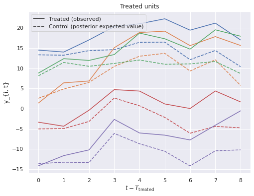
Here we see that the posterior estimates of the treatment effect are quite close to the actual effect.
fig, ax = plt.subplots(figsize=(8, 6))

low, high = (
    (y[treated, T_treat:] - post_treat_ctrl)
        .quantile([0.025, 0.975],
                  dim=("chain", "draw", "treat_unit"))
)
ax.fill_between(np.arange(T - T_treat), low, high,
                color='C0', alpha=0.25,
                label="95% credible interval");
ax.plot([0, T - T_treat - 1], [0, T - T_treat - 1],
        c='k', label="Actual");
ax.plot(
    y[treated, T_treat:].T \
        - post_treat_ctrl.mean(dim=("chain", "draw")).T,
    c='C0'
);

handles, _ = ax.get_legend_handles_labels()
handles.insert(
    1, Line2D([0], [0],c='C0', label="Posterior expected")
)
ax.legend(loc='upper left', handles=handles);

ax.set_xlabel(r"$t - T_{\mathrm{treated}}$");
ax.set_ylabel("Treatment effect");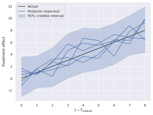
This post is available as a Jupyter notebook here.
Pang, Xun, Licheng Liu, and Yiqing Xu. “A Bayesian alternative to synthetic control for comparative case studies.” Available at SSRN (2020).↩︎
Murphy, Kevin P. Machine learning: a probabilistic perspective. MIT press, 2012.↩︎