The Hierarchical Regularized Horseshoe Prior in PyMC3

For some time I have been interested in better understanding the horseshoe prior¹ by implementing it in PyMC3. The horsehoe prior is a continuous alternative to the spike-and-slab prior for sparse Bayesian estimation. The continuity of the horeshoe prior allows for simpler estimation using general purpose Bayesian computation packages such as pymc3 and Stan. Piironen and Vehtari² have proposed a hierarchical regularized horseshoe prior that has advantages over the original horseshoe prior when it comes to specifying the hyperprior distributions on the regularization parameters. In the appendix of their paper, Piironen and Vehtari give a sample implementation in Stan. This post gives a corresponding implementation in pymc3 and tests it on simulated data.

First we import the necessary Python packages and do some light housekeeping.

%matplotlib inline

from warnings import filterwarnings

from aesara import tensor as at
import arviz as az
from matplotlib import pyplot as plt
import numpy as np
import pymc3 as pm
import seaborn as sns

filterwarnings('ignore', category=UserWarning, module='aesara')
filterwarnings('ignore', category=UserWarning, module='arviz')

sns.set(color_codes=True)

Simulated Data

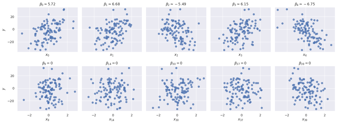
Since the horseshoe is designed for sparse estimation of regression parameters, we simulate data from a model with \(D = 50\) variables, \(D_0 = 5\) of which are nonzero.

D = 50
D0 = 5

SEED = 123456789 # for reproducibility

rng = np.random.default_rng(SEED)

INTERCEPT = rng.uniform(-3, 3)

COEF = np.zeros(D)
COEF[:D0] = rng.choice([-1, 1], size=D0) * rng.normal(5, 1, size=D0)

Now we draw \(N = 100\) random observations with \(x_i \sim N(0, 1).\)

N = 100

X = rng.normal(size=(N, D))

We now simulate responses from this regression model with \(N(0, 1)\)-distributed noise.

SIGMA = 1.

y = INTERCEPT + X.dot(COEF) + rng.normal(0, SIGMA, size=N)

We see that there is a linear relationship between \(y\) and the first \(D_0\) variables and no relationship between \(y\) and a random sample from the subsequent \(D - D0\) variables.

fig, axes = plt.subplots(nrows=2, ncols=D0,
                         sharex=True, sharey=True,
                         figsize=(16, 6))

for i, (ax, coef) in enumerate(zip(axes[0], COEF)):
    ax.scatter(X[:, i], y, alpha=0.75);
    
    ax.set_xlabel(f"$x_{{ {i} }}$");
    ax.set_title(f"$\\beta_{{ {i} }} \\approx {coef:.2f}$");


zero_coef_ix = rng.choice(range(D0, D), replace=False, size=D0)
zero_coef_ix.sort()

for ax, i in zip(axes[1], zero_coef_ix):
    ax.scatter(X[:, i], y, alpha=0.75);
    
    ax.set_xlabel(f"$x_{{ {i} }}$");
    ax.set_title(f"$\\beta_{{ {i} }} = 0$");
    
axes[0, 0].set_ylabel("$y$");
axes[1, 0].set_ylabel("$y$");

fig.tight_layout();

The Regularized Horseshoe

First we place a reasonable half-normal prior on the error variance \(\sigma^2\).

with pm.Model() as model:
    σ = pm.HalfNormal("σ", 2.5)

The hierarchical regularized horseshoe uses two levels of regularization, global and local. There is a global parameter, \(\tau\), that will shrink all parameters towards zero (similarly to ridge regression) along with local parameters \(\lambda_i\) for each coefficient. A long-tailed prior on the \(\lambda_i\)s allows some of them to be nonzero, with the scale of \(\tau\) setting the prior expected number of nonzero parameters.

An important calculation (§3.3 of Piironen and Vehtari) shows that if we believe there are actually \(D_*\) nonzero coefficients, the prior on the global shrinkage parameter \(\tau\) should be

\[ \tau \sim \textrm{Half-StudentT}_{2} \left(\frac{D_*}{D - D_*} \cdot \frac{\sigma}{\sqrt{N}}\right). \]

Since we know the generating process for this data, we set \(D_* = D_0\), although Piironen and Vehtari show that this guess only needs to be order-of-magnitude correct in practice.

with model:
    τ = pm.HalfStudentT("τ", 2, D0 / (D - D0) * σ / np.sqrt(N))

The regularized horseshoe uses the prior

\[\beta_i \sim N\left(0, \tau^2 \cdot \tilde{\lambda}_i^2\right)\]

for the coefficients, where

\[\tilde{\lambda}_i^2 = \frac{c^2 \lambda_i^2}{c^2 + \tau^2 \lambda_i^2}.\]

Given these definitions, it only remains to specify priors on \(\lambda_i\) and \(c\). As indicated above, we use a long-tailed prior \(\lambda_i \sim \textrm{Half-StudentT}_5(1)\) on the local parameters

with model:
    λ = pm.HalfStudentT("λ", 5, shape=D)

Following §2.3 of Piironen and Vehtari, we place an inverse gamma prior on \(c^2\), \(c^2 \sim \textrm{InverseGamma}(1, 1).\)

with model:
    c2 = pm.InverseGamma("c2", 1, 1)

With these priors in place, we define \(\tilde{\lambda}_i\)

with model:
    λ_ = λ * at.sqrt(c2 / (c2 + τ**2 * λ**2))

To implement \(\beta_i \sim N\left(0, \tau^2 \cdot \tilde{\lambda}_i^2\right)\) more efficiently, we use the parameterization

\[ \begin{align*} z_i & \sim N(0, 1), \\ \beta_i & = z_i \cdot \tau \cdot \tilde{\lambda_i}. \end{align*} \]

with model:
    z = pm.Normal("z", 0., 1., shape=D)
    β = pm.Deterministic("β", z * τ * λ_)

Note that it is important to constrain two of the three factors \(z_i\), \(\tau\), and \(\tilde{\lambda}_i\) to be positive, otherwise this model will not be fully identified. Unlike in Piironen and Vehtari, we enforce identifiability by using half-Student T priors on \(\tau\) and \(\lambda_i\).

Using a relatively flat \(N(0, 10^2)\) prior for the intercept, the likelihood of the observed data is

with model:
    β0 = pm.Normal("β0", 0, 10.)
    
    obs = pm.Normal("obs", β0 + at.dot(X, β), σ, observed=y)

We proceed to sample from this model

CHAINS = 3

SAMPLE_KWARGS = {
    'cores': CHAINS,
    'target_accept': 0.99,
    'max_treedepth': 15,
    'random_seed': [SEED + i for i in range(CHAINS)],
    'return_inferencedata': True
}

with model:
    trace = pm.sample(**SAMPLE_KWARGS)

Auto-assigning NUTS sampler...
Initializing NUTS using jitter+adapt_diag...
Multiprocess sampling (3 chains in 3 jobs)
NUTS: [β0, z, c2, λ, τ, σ]

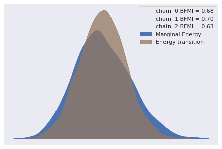
Sampling 3 chains for 1_000 tune and 1_000 draw iterations (3_000 + 3_000 draws total) took 322 seconds.

The energy plot, BFMIs, and \(\hat{R}\) statistics for these samples show no cause for concern.

az.plot_energy(trace);

az.rhat(trace).max()

<xarray.Dataset>
Dimensions:  ()
Data variables:
    z        float64 1.006
    β0       float64 1.001
    σ        float64 1.001
    τ        float64 1.002
    λ        float64 1.004
    c2       float64 1.0
    β        float64 1.002

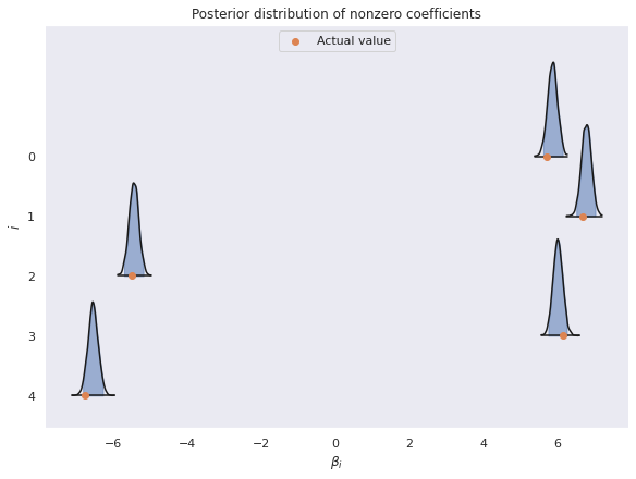
The relative error in recovering the true nonzero parameters is quite good (the largest relative error is approximately 3%).

def post_mean(trace, var_name):
    return trace["posterior"][var_name].mean(dim=("chain", "draw"))

np.abs((post_mean(trace, "β")[:D0] - COEF[:D0]) / COEF[:D0]).max()

<xarray.DataArray 'β' ()>
array(0.03201216)

Visually, the true parameter values lie comfortably inside the 95% high posterior density intervals for these nonzero parameters.

ax, = az.plot_forest(
    trace, var_names=["β"], coords={"β_dim_0": range(D0)},
    kind='ridgeplot', ridgeplot_truncate=False, ridgeplot_alpha=0.5,
    hdi_prob=0.95, combined=True,
    figsize=(8, 6)
)
ax.scatter(COEF[:D0][::-1], ax.get_yticks(),
           c='C1',
           label="Actual value");

ax.set_xlabel(r"$\beta_i$");

ax.set_ylim(bottom=None, top=1.55 * ax.get_yticks().max())
ax.set_yticklabels(range(D0)[::-1]);
ax.set_ylabel(r"$i$");

ax.legend(loc='upper center');
ax.set_title("Posterior distribution of nonzero coefficients");

The (absolute) largest posterior expected value for a coefficient that is actually zero is relatively small compared to the scale of the nonzero parameters.

np.abs(post_mean(trace, "β")[D0:]).max()

<xarray.DataArray 'β' ()>
array(0.2778543)

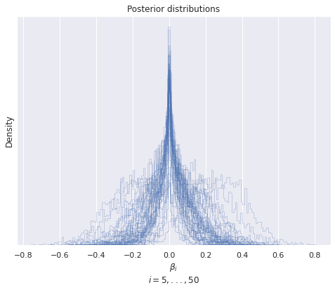
The following plot shows the posterior distributions of the \(D - D_0 = 45\) coefficients. Most of the distributions show a pronounced peak around zero, as we would expect for a sparse estimator.

fig, ax = plt.subplots(figsize=(8, 6))

for i in range(D0, D):
    ax.hist(trace["posterior"]["β"][..., i].data.ravel(),
            histtype='step', bins=100,
            color='C0', alpha=0.25,);

ax.set_xlabel(f"$\\beta_i$\n$i = {D0},...,{D}$");

ax.set_yticks([]);
ax.set_ylabel("Density");

ax.set_title("Posterior distributions");

And surely enough, all but one of the 95% high posterior density intervals for the coefficients that are actually zero contain zero.

post_β_low, post_β_high = trace["posterior"]["β"][..., D0:].quantile([0.025, 0.975], dim=('chain', 'draw'))

((post_β_low <= 0) & (0 <= post_β_high)).mean()

<xarray.DataArray 'β' ()>
array(0.97777778)

This post is available as a Jupyter notebook here.

Many thanks to Sue Márquez for pointing out that the original post spelled Aki’s name wrong, and sincere apologies to Aki.

%load_ext watermark
%watermark -n -u -v -iv

Last updated: Sat May 29 2021

Python implementation: CPython
Python version       : 3.8.8
IPython version      : 7.22.0

matplotlib: 3.4.1
arviz     : 0.11.2
numpy     : 1.20.2
pymc3     : 3.11.1
aesara    : 2.0.6
seaborn   : 0.11.1