A PyMC3 Analysis of Tyrannosaurid Growth Curves
In Chapter 7 of their excellent book Bayesian Statistical Methods (BSM from now on), Reich and Ghosh work an example analysis of the growth rates of Tyrannosaurids in R using JAGS. This dataset and analysis are quite fun, so this post shows how to execute (almost) the same analysis in Python using PyCM3.
The Dataset
To quote BSM,
We analyze the data from 20 fossils to estimate the growth curves of four tyrannosaurid species: Albertosaurus, Daspletosaurus, Gorgosaurus and Tyrannosaurus. The data are taken from Table 1 of Erickson, GM et al (2004).
First we make some standard Python imports and load the dataset from the author’s website.
%matplotlib inlinefrom warnings import filterwarningsfrom aesara import shared, tensor as at
import arviz as az
from matplotlib import MatplotlibDeprecationWarning, pyplot as plt
import numpy as np
import pandas as pd
import pymc3 as pm
import seaborn as snsfilterwarnings('ignore', category=UserWarning, module='aesara')
filterwarnings('ignore', category=UserWarning, module='arviz')
filterwarnings('ignore', category=MatplotlibDeprecationWarning, module='pandas')sns.set(color_codes=True)%%bash
DATA_URI=https://www4.stat.ncsu.edu/~bjreich/BSMdata/Erickson.csv
DATA_DEST=/tmp/Erickson.csv
if [[ ! -e $DATA_DEST ]];
then
wget -q -O $DATA_DEST $DATA_URI
fidf = (pd.read_csv('/tmp/Erickson.csv')
.rename(columns=str.lower)
.sort_values('age')
.reset_index(drop=True))df.head()| taxon | spec. # | age | mass | |
|---|---|---|---|---|
| 0 | Albertosaurus | RTMP 2002.45.46 | 2 | 50.3 |
| 1 | Tyrannosaurus | LACM 28471 | 2 | 29.9 |
| 2 | Gorgosaurus | FMNH PR2211 | 5 | 127.0 |
| 3 | Gorgosaurus | RTMP 86.144.1 | 7 | 229.0 |
| 4 | Daspletosaurus | RTMP 94.143.1 | 10 | 496.0 |
Exploratory data analysis
First we summarize and plot the data.
df.describe()| age | mass | |
|---|---|---|
| count | 20.00000 | 20.000000 |
| mean | 15.10000 | 1568.760000 |
| std | 7.05542 | 1562.465702 |
| min | 2.00000 | 29.900000 |
| 25% | 13.00000 | 579.250000 |
| 50% | 15.50000 | 1123.500000 |
| 75% | 18.75000 | 1795.000000 |
| max | 28.00000 | 5654.000000 |
grid = sns.catplot(x='age', y='mass', hue='taxon', data=df)

grid.ax.set_xlim(left=1);
grid.ax.set_xscale('log');

grid.ax.set_ylim(bottom=100);
grid.ax.set_yscale('log');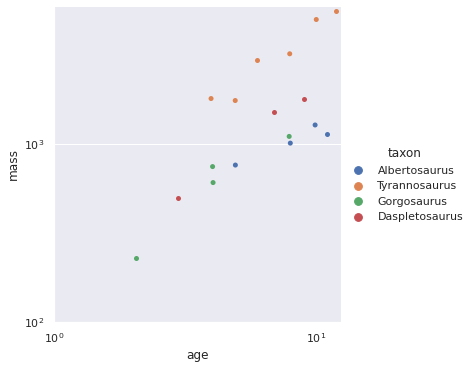
Note the logarithmic scale on both of the axes here. A few points are immediately apparent.
- There are only 20 samples, so the data is fairly small.
- Mass varies fairly widely across taxa.
- The relationship between age and mass appears linear on the log-log scale.
- Variance appears to increase with age.
Modeling
Given the third and fourth observations about the data,
[w]e use multiplicative error rather than additive error because variation in the population likely increases with mass/age.
Throughout this post \(Y_i\) and \(X_i\) will correspond to the mass and age of the \(i\)-th sample respectively. Each of our four models will take the form
\[Y_i = f_{j(i)}(X_i) \cdot \varepsilon_{j(i)}.\]
Here \(\varepsilon_j\) corresponds to the multiplicative error for the \(j\)-th taxon and \(j(i)\) is the taxon identifier of the \(i\)-th sample.
We place a log-normal prior on \(\varepsilon_j\) so that $ (_j) = 1$ and \(\textrm{Var}\left(\log(\varepsilon_j)\right) = \sigma_j^2\). With the notation \(y_i = \log Y_i\) and \(x_i = \log X_i\), standard distributional math shows that
\[y_i \sim N\left(\log\left(f_{j(i)}(X_{j(i)})\right) - \frac{\sigma_{j(i)}^2}{2}, \sigma_{j(i)}^2\right).\]
Each of the four models we consider arises from a choice of the form of \(f_j(X)\) (along with a prior for any of its unknown parameters) and a prior on \(\sigma_j\).
Unpooled log-linear model
Given the third observation above, we begin with a log-linear model for the relationship between age and mass. If
\[f_j(X) = A_j \cdot X^{b_j}\]
then
\[\log\left(f_j(X)\right) = a_j + b_j \log X,\]
where \(a_j = \log A_j\).
We define log_age and log_mass which correspond to \(x_i\) and \(y_i\) respectively.
log_age = np.log(df['age'].values)
log_mass = np.log(df['mass'].values)
We turn the taxon names into numeric identifiers and set up shared containers for log_age and taxon_id. These shared containers are aesara’s way to facilitate posterior predictive sampling. aesara is the PyMC team’s fork of theano. Since active development on theano has ceased, pymc3 now uses aesara for tensor calculations.
taxon_id, taxon_map = df['taxon'].factorize(sort=True)
n_taxon = taxon_map.size
taxon_id_ = shared(taxon_id)
log_age_ = shared(log_age)Given the second observation above, we will actually specify one model per taxon (hence the adjective “unpooled”). This model has regression coefficients
\[ \begin{align*} a_j & \sim N(0, 2.5^2) \\ b_j & \sim N(0, 2.5^2). \end{align*} \]
with pm.Model() as loglin_model:
    a = pm.Normal("a", 0., 2.5, shape=n_taxon)
    b = pm.Normal("b", 0., 2.5, shape=n_taxon)
Note that these prior differs differ slightly (in their variance) from those in the BSM. Nevertheless, the results will be quite similar. With the prior on \(\sigma_j \sim N(0, 2.5^2)\), we can finish specifying the model in code.
with loglin_model:
    σ = pm.HalfNormal("σ", 2.5, shape=n_taxon)
    μ = a[taxon_id_] + b[taxon_id_] * log_age_ - 0.5 * σ[taxon_id_]**2

    obs = pm.Normal("obs", μ, σ[taxon_id_], observed=log_mass)
We now sample from the posterior distribution of the model.
CHAINS = 3
DRAWS = 2000
SEED = 12345 # for reproducibility

SAMPLE_KWARGS = {
    'cores': CHAINS,
    'draws': DRAWS,
    'random_seed': [SEED + i for i in range(CHAINS)],
    'return_inferencedata': True,
    'target_accept': 0.995
}
with loglin_model:
loglin_trace = pm.sample(**SAMPLE_KWARGS)Auto-assigning NUTS sampler...
Initializing NUTS using jitter+adapt_diag...
Multiprocess sampling (3 chains in 3 jobs)
NUTS: [σ, b, a]100.00% [9000/9000 03:15<00:00 Sampling 3 chains, 0 divergences]
Sampling 3 chains for 1_000 tune and 2_000 draw iterations (3_000 + 6_000 draws total) took 198 seconds.
The number of effective samples is smaller than 25% for some parameters.
To check that there is no obvious problem with our samples we check the energy plot, Bayesian fraction of missing information (BFMI), and Gelman-Rubin statistics.
az.plot_energy(loglin_trace);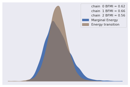
Since the marginal and transitional energy distributions are similar and each BFMI is greater than 0.2, these diagnostics show no obvious issues.
az.rhat(loglin_trace).max()<xarray.Dataset>
Dimensions: ()
Data variables:
a float64 1.008
b float64 1.006
σ float64 1.003
-
-
-
-
a()float641.008
array(1.00765472)
-
b()float641.006
array(1.00622094)
-
σ()float641.003
array(1.00281897)
-
-
The Gelman-Rubin statistics for each parameter are acceptable (smaller than 1.05) as well.
We now draw samples from the posterior predictive distribution of \(Y\). First we build a grid for \(x\) (pp_log_age) and \(j\) (pp_taxon_id) that span the observed range of these quantities in the data.
pp_log_age = np.repeat(np.linspace(0, np.log(30)), n_taxon)
pp_taxon_id = np.tile(np.arange(n_taxon), pp_log_age.size // n_taxon)
Now we sample from the posterior predictive distribution.
ALPHA = 0.05def get_pp_df(model, trace, alpha=ALPHA):
taxon_id_.set_value(pp_taxon_id)
log_age_.set_value(pp_log_age)
with model:
pp_trace = pm.sample_posterior_predictive(trace)
taxon_id_.set_value(taxon_id)
log_age_.set_value(log_age)
return pd.DataFrame({
'age': np.exp(pp_log_age),
'taxon_id': pp_taxon_id,
'pp_mean': np.exp(pp_trace['obs'].mean(axis=0)),
'pp_low': np.exp(np.percentile(pp_trace['obs'], 100 * alpha / 2., axis=0)),
'pp_high': np.exp(np.percentile(pp_trace['obs'], 100 * (1 - alpha / 2.), axis=0))
})Note the lines in get_pp_df where we change the values of the shared variables taxon_id_ and log_age_ to their posterior predictive grid values before sampling and back to the observed values after sampling.
pp_loglin_df = get_pp_df(loglin_model, loglin_trace)100.00% [6000/6000 00:31<00:00]
pp_loglin_df.head()| age | taxon_id | pp_mean | pp_low | pp_high | |
|---|---|---|---|---|---|
| 0 | 1.000000 | 0 | 19.767345 | 7.513964 | 44.358809 |
| 1 | 1.000000 | 1 | 3.751587 | 0.029910 | 96.423621 |
| 2 | 1.000000 | 2 | 8.544977 | 2.598875 | 22.385467 |
| 3 | 1.000000 | 3 | 7.263371 | 2.957169 | 17.696855 |
| 4 | 1.071878 | 0 | 21.720457 | 8.950703 | 48.788518 |
Finally, after all of this preparatory work, we get to the payoff and plot the posterior predictive means and intervals for each taxon across our grid.
def make_posterior_mean_label(name):
    return "Posterior mean" if name is None else f"{name}\nposterior mean"

def make_posterior_interval_label(name):
    return "95% interval" if name is None else f"{name}\n95% interval"

def plot_taxon_posterior(taxon, df, pp_df,
                         name=None, plot_data=True,
                         legend=True, ax=None):
    if ax is None:
        fig, ax = plt.subplots(figsize=(8, 6))

    ax.fill_between(pp_df['age'], pp_df['pp_low'], pp_df['pp_high'],
                    alpha=0.25, label=make_posterior_interval_label(name));
    pp_df.plot('age', 'pp_mean', label=make_posterior_mean_label(name), ax=ax)

    if plot_data:
        df.plot.scatter('age', 'mass', c='C0', label="Data", ax=ax)

    ax.set_title(taxon)

    if legend:
        ax.legend(loc=2)
    else:
        ax.get_legend().remove()

    return ax
FIGSIZE = (12, 9)def plot_pp_by_taxon(pp_df,
name=None, plot_data=True,
fig=None, axes=None, figsize=FIGSIZE):
if fig is None or axes is None:
fig, axes = plt.subplots(nrows=2, ncols=2, sharex=True, sharey=True, figsize=figsize)
for plt_taxon_id, ax in enumerate(axes.flatten()):
taxon = taxon_map[plt_taxon_id]
taxon_df = df[taxon_id == plt_taxon_id]
taxon_pp_df = pp_df[pp_df['taxon_id'] == plt_taxon_id]
plot_taxon_posterior(taxon, taxon_df, taxon_pp_df,
name=name, plot_data=plot_data,
legend=(plt_taxon_id == 0), ax=ax)
ax.set_xlim(right=30)
ax.set_ylim(top=6000)
return fig, axesplot_pp_by_taxon(pp_loglin_df);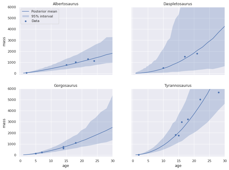
Visually comparing these plots to the corresponding ones in the worked JAGS example shows reasonable agreement in spite of our slightly different prior specification.
Pooled log-linear model
It is quite noticeable that in the above posterior predictive plots that the credible intervals are wider for taxa that have fewer data points. In particular there are only three samples of taxon Daspletosaurus. A hierarchical model will allow us to share information from taxa with more observations when inferring the posterior distributions of parameters for taxa with fewer observations. This information sharing leads to the use of the term “pooled” for this type of model. The pooled log linear model still takes the form
\[\log\left(f_j(X)\right) = a_j + b_j \log X,\]
but uses different priors on \(a_j\) and \(b_j\). Conceptually, the pooled model uses the priors
\[ \begin{align*} \mu_a & \sim N(0, 2.5^2) \\ \sigma_a & \sim \textrm{HalfNormal}(2.5^2) \\ a_j & \sim N(\mu_a, \sigma_a^2), \end{align*} \]
and similarly for \(b_j\).
In reality, this intuitive parameterization can often present computational challenges, so we use the following non-centered parameterization instead.
\[ \begin{align*} \mu_a & \sim N(0, 2.5^2) \\ \Delta_{a_j} & \sim N(0, 1) \\ \sigma_a & \sim \textrm{HalfNormal}(2.5^2) \\ a_j & = \mu_a + \Delta_{a_j} \cdot \sigma_a. \end{align*} \]
def hierarchical_normal(name, shape):
    μ = pm.Normal(f"μ_{name}", 0., 2.5)
    Δ = pm.Normal(f"Δ_{name}", 0., 1., shape=shape)
    σ = pm.HalfNormal(f"σ_{name}", 2.5)

    return pm.Deterministic(name, μ + Δ * σ)
with pm.Model() as pooled_loglin_model:
a = hierarchical_normal("a", n_taxon)
b = hierarchical_normal("b", n_taxon)To further share information across taxa, we enforce the constraint that the noise parameters are identical across taxa, \(\sigma_1 = \sigma_2 = \sigma_3 = \sigma_4 = \sigma\), with the prior \(\sigma \sim \textrm{HalfNormal}(2.5^2)\).
with pooled_loglin_model:
    σ = pm.HalfNormal("σ", 2.5)
    μ = a[taxon_id_] + b[taxon_id_] * log_age_ - 0.5 * σ**2

    obs = pm.Normal("obs", μ, σ, observed=log_mass)
We now sample from the pooled log-linear model.
with pooled_loglin_model:
    pooled_loglin_trace = pm.sample(**SAMPLE_KWARGS)
Auto-assigning NUTS sampler...
Initializing NUTS using jitter+adapt_diag...
Multiprocess sampling (3 chains in 3 jobs)
NUTS: [σ, σ_b, Δ_b, μ_b, σ_a, Δ_a, μ_a]100.00% [9000/9000 08:33<00:00 Sampling 3 chains, 0 divergences]
Sampling 3 chains for 1_000 tune and 2_000 draw iterations (3_000 + 6_000 draws total) took 514 seconds.
The number of effective samples is smaller than 25% for some parameters.
Again our diagnostics show no obvious cause for concern.
az.plot_energy(pooled_loglin_trace);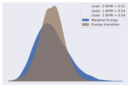
az.rhat(pooled_loglin_trace).max()<xarray.Dataset>
Dimensions: ()
Data variables:
μ_a float64 1.002
Δ_a float64 1.002
μ_b float64 1.0
Δ_b float64 1.001
σ_a float64 1.002
a float64 1.002
σ_b float64 1.004
b float64 1.002
σ float64 1.006
-
-
-
-
μ_a()float641.002
array(1.00208566)
-
Δ_a()float641.002
array(1.00184228)
-
μ_b()float641.0
array(1.00044944)
-
Δ_b()float641.001
array(1.00108353)
-
σ_a()float641.002
array(1.00158498)
-
a()float641.002
array(1.00175827)
-
σ_b()float641.004
array(1.00390892)
-
b()float641.002
array(1.00210233)
-
σ()float641.006
array(1.00598006)
-
-
Again we sample from the posterior predictive distribution of this model and plot the results.
pp_pooled_loglin_df = get_pp_df(pooled_loglin_model, pooled_loglin_trace)100.00% [6000/6000 00:52<00:00]
pp_pooled_loglin_df.head()| age | taxon_id | pp_mean | pp_low | pp_high | |
|---|---|---|---|---|---|
| 0 | 1.000000 | 0 | 17.405405 | 9.378821 | 30.602004 |
| 1 | 1.000000 | 1 | 9.940230 | 3.453810 | 27.524651 |
| 2 | 1.000000 | 2 | 9.484354 | 4.619197 | 18.747739 |
| 3 | 1.000000 | 3 | 8.394668 | 4.823675 | 15.338217 |
| 4 | 1.071878 | 0 | 19.095916 | 10.369680 | 33.178229 |
plot_pp_by_taxon(pp_pooled_loglin_df);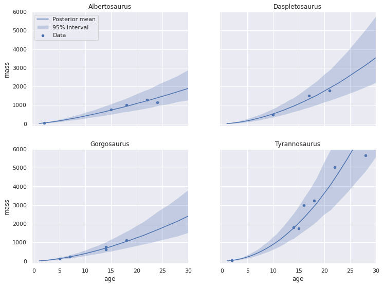
Visually, each of the credible intervals appears smaller than for the unpooled model, espescially for Daspletosaurus. We can overlay the posterior predictive plots for the unpooled and pooled log-linear models to confirm this observation.
fig, axes = plot_pp_by_taxon(pp_loglin_df, plot_data=False, name="Unpooled log-linear")
plot_pp_by_taxon(pp_pooled_loglin_df,
                 name="Pooled log-linear",
                 fig=fig, axes=axes);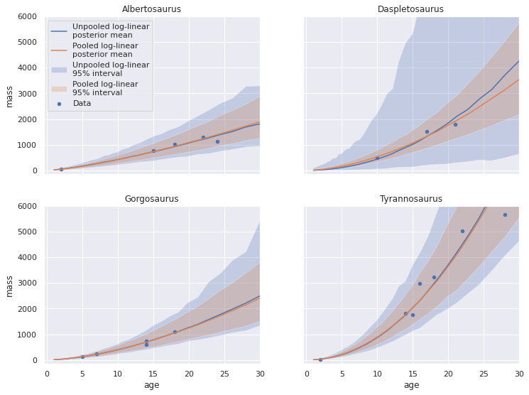
Unpooled logistic model
While the log-linear models are reasonable given our exploratory data analysis above (and produce visually plausible results), they are physically unrealistic. With a log-linear model, as the dinosaur gets older its mass will increase without bound. In reality, living creatures have a maximum lifespan, so the log-linear model may be reasonable for realistic ages. Nevertheless, we can incorporate upper bounds on mass by using a logistic function for \(f_j\),
\[f_j(x) = a_j + \frac{b_j}{1 + \exp\left(-(x - c_j)\ /\ d_j\right)}\]
def logistic(x, a, b, c, d, tensor=False):
    exp = at.exp if tensor else np.exp

    return a + b / (1. + exp(-(x - c) / d))

def inv_logistic(y, a, b, c, d, tensor=False):
    log = at.log if tensor else np.log

    return c - d * log(b / (y - a) - 1)
Note that logistic and its inverse function, inv_logistic, switch between the aesera and numpy implementations of exp and log depending on the tensor parameter.
fig, ax = plt.subplots(figsize=(8, 6))

A, B, C, D = 1, 5, 10, 3

f = lambda x: logistic(x, A, B, C, D)
f_inv = lambda y: inv_logistic(y, A, B, C, D)

X_MAX = f_inv(A + B - 0.01)
logistic_x = np.linspace(0, X_MAX)

ax.plot(logistic_x, f(logistic_x));

ax.set_xlim(0, X_MAX);

ax.set_yticks([0, f(0), f(2 * X_MAX)]);
ax.set_yticklabels(["0", r"$f(0)$",
                    r"$\lim_{x \to \infty}\ f(x)$"]);

ax.set_title(f"Logistic function $f$ with\n$a =${A}, $b =${B}, $c =${C}, $d =${D}");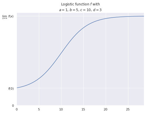
We require \(a, b, d > 0\), so we set
\[ \begin{align*} a_j & = \exp \alpha_j \\ b_j & = \exp \beta_j \\ d_j & = \exp \delta_j. \end{align*} \]
For the unpooled logistic model we use \(\alpha_j \sim N(0, 2.5^2)\) and similarly for \(\beta_j\) and \(\delta_j\). We use the same prior for \(c_j\) as in the unpooled log-linear model.
with pm.Model() as logistic_model:
    α = pm.Normal("α", 0., 2.5, shape=n_taxon)
    a = pm.Deterministic("a", at.exp(α))

    β = pm.Normal("β", 0., 2.5, shape=n_taxon)
    b = pm.Deterministic("b", at.exp(β))

    c = pm.Normal("c", 0., 2.5, shape=n_taxon)

    δ = pm.Normal("δ", 0., 2.5, shape=n_taxon)
    d = pm.Deterministic("d", at.exp(δ))
The noise variance is also the same as in the unpooled log-linear model. The likelihood is quite similar as well.
with logistic_model:
    σ = pm.HalfNormal("σ", 2.5, shape=n_taxon)
    μ = at.log(
            logistic(log_age_,
                     a[taxon_id_], b[taxon_id_], c[taxon_id_], d[taxon_id_],
                     tensor=True)
        ) - 0.5 * σ[taxon_id_]**2

    obs = pm.Normal("obs", μ, σ[taxon_id_], observed=log_mass)
We now sample from the unpooled logistic model.
with logistic_model:
    logistic_trace = pm.sample(**SAMPLE_KWARGS)
Auto-assigning NUTS sampler...
Initializing NUTS using jitter+adapt_diag...
Multiprocess sampling (3 chains in 3 jobs)
NUTS: [σ, δ, c, β, α]100.00% [9000/9000 09:42<00:00 Sampling 3 chains, 13 divergences]
Sampling 3 chains for 1_000 tune and 2_000 draw iterations (3_000 + 6_000 draws total) took 583 seconds.
There were 2 divergences after tuning. Increase `target_accept` or reparameterize.
The chain reached the maximum tree depth. Increase max_treedepth, increase target_accept or reparameterize.
There were 6 divergences after tuning. Increase `target_accept` or reparameterize.
There were 5 divergences after tuning. Increase `target_accept` or reparameterize.
The estimated number of effective samples is smaller than 200 for some parameters.
Again our diagnostics show no obvious cause for concern.
az.plot_energy(logistic_trace);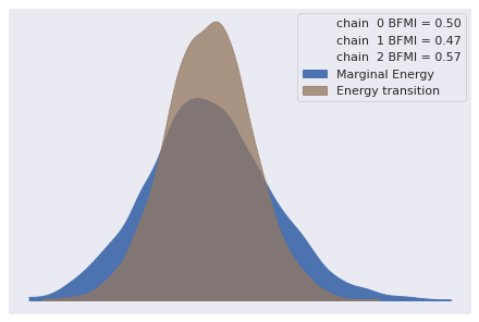
az.rhat(logistic_trace).max()<xarray.Dataset>
Dimensions: ()
Data variables:
α float64 1.017
β float64 1.02
c float64 1.008
δ float64 1.008
a float64 1.017
b float64 1.02
d float64 1.014
σ float64 1.024
-
-
-
-
α()float641.017
array(1.01676666)
-
β()float641.02
array(1.02040336)
-
c()float641.008
array(1.00824226)
-
δ()float641.008
array(1.00846537)
-
a()float641.017
array(1.01676666)
-
b()float641.02
array(1.02040336)
-
d()float641.014
array(1.0135121)
-
σ()float641.024
array(1.02389979)
-
-
Again we sample from the posterior predictive distribution of this model and plot the results.
pp_logistic_df = get_pp_df(logistic_model, logistic_trace)100.00% [6000/6000 00:35<00:00]
pp_logistic_df.head()| age | taxon_id | pp_mean | pp_low | pp_high | |
|---|---|---|---|---|---|
| 0 | 1.000000 | 0 | 20.229437 | 0.655100 | 809.706349 |
| 1 | 1.000000 | 1 | 372.903045 | 0.370631 | 5551.674728 |
| 2 | 1.000000 | 2 | 60.408886 | 0.477719 | 1983.882017 |
| 3 | 1.000000 | 3 | 11.421099 | 1.119319 | 53.975799 |
| 4 | 1.071878 | 0 | 21.909702 | 0.812396 | 642.989663 |
fig, axes = plot_pp_by_taxon(pp_loglin_df, name="Unpooled log-linear")
plot_pp_by_taxon(pp_logistic_df,
                 name="Unpooled logistic",
                 fig=fig, axes=axes);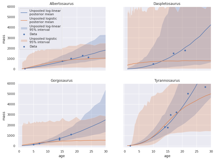
Interestingly, the posterior predictive mean for Daspletosaurus doesn’t seem to fit the observed data as well as the log-linear model, and the credible intervals are quite wide. This observation makes sense given that the logistic model has twice as many parameters, but the number of observations has remained the same.
Pooled logistic
We can once again share information across taxa by specifying a pooled logistic model. This model places hierarchical normal priors on \(\alpha\), \(\beta\), \(c\), and \(\delta\).
with pm.Model() as pooled_logistic_model:
    α = hierarchical_normal("α", n_taxon)
    a = pm.Deterministic("a", at.exp(α))

    β = hierarchical_normal("β", n_taxon)
    b = pm.Deterministic("b", at.exp(β))

    c = hierarchical_normal("c", n_taxon)

    δ = hierarchical_normal("δ", n_taxon)
    d = pm.Deterministic("d", at.exp(δ))
The noise variance and likelihood are similar to those of the unpooled logistic model, except we constrain all taxa to share the same noise variance, \(\sigma\), as in the pooled log-linear model.
with pooled_logistic_model:
    σ = pm.HalfNormal("σ", 2.5)
    μ = at.log(
            logistic(log_age_,
                     a[taxon_id_], b[taxon_id_], c[taxon_id_], d[taxon_id_],
                     tensor=True)
        ) - 0.5 * σ**2

    obs = pm.Normal("obs", μ, σ, observed=log_mass)
with pooled_logistic_model:
pooled_logistic_trace = pm.sample(**SAMPLE_KWARGS)Auto-assigning NUTS sampler...
Initializing NUTS using jitter+adapt_diag...
Multiprocess sampling (3 chains in 3 jobs)
NUTS: [σ, σ_δ, Δ_δ, μ_δ, σ_c, Δ_c, μ_c, σ_β, Δ_β, μ_β, σ_α, Δ_α, μ_α]100.00% [9000/9000 19:02<00:00 Sampling 3 chains, 3 divergences]
Sampling 3 chains for 1_000 tune and 2_000 draw iterations (3_000 + 6_000 draws total) took 1143 seconds.
There were 2 divergences after tuning. Increase `target_accept` or reparameterize.
There was 1 divergence after tuning. Increase `target_accept` or reparameterize.
Again our diagnostics show no obvious cause for concern.
az.plot_energy(pooled_logistic_trace);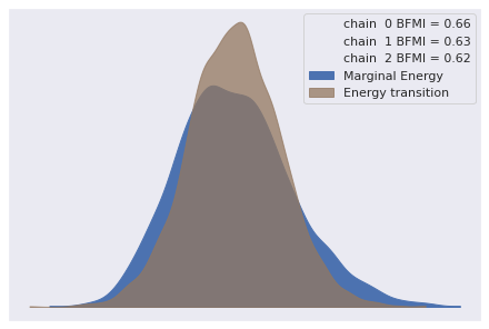
(az.rhat(pooled_logistic_trace['posterior'])
   .max()
   .to_array()
   .max())
<xarray.DataArray ()> array(1.00208561)
-
1.002
array(1.00208561)
-
-
Again we sample from the posterior predictive distribution of this model and plot the results.
pp_pooled_logistic_df = get_pp_df(pooled_logistic_model, pooled_logistic_trace)100.00% [6000/6000 01:08<00:00]
pp_pooled_logistic_df.head()| age | taxon_id | pp_mean | pp_low | pp_high | |
|---|---|---|---|---|---|
| 0 | 1.000000 | 0 | 22.852762 | 10.267422 | 56.497339 |
| 1 | 1.000000 | 1 | 9.839328 | 0.906120 | 125.299677 |
| 2 | 1.000000 | 2 | 12.589540 | 3.182979 | 91.279583 |
| 3 | 1.000000 | 3 | 11.080350 | 4.344195 | 36.627854 |
| 4 | 1.071878 | 0 | 24.465512 | 11.729286 | 56.373575 |
fig, axes = plot_pp_by_taxon(pp_logistic_df, plot_data=False, name="Unpooled logistic")
plot_pp_by_taxon(pp_pooled_logistic_df,
                 name="Pooled logistic",
                 fig=fig, axes=axes);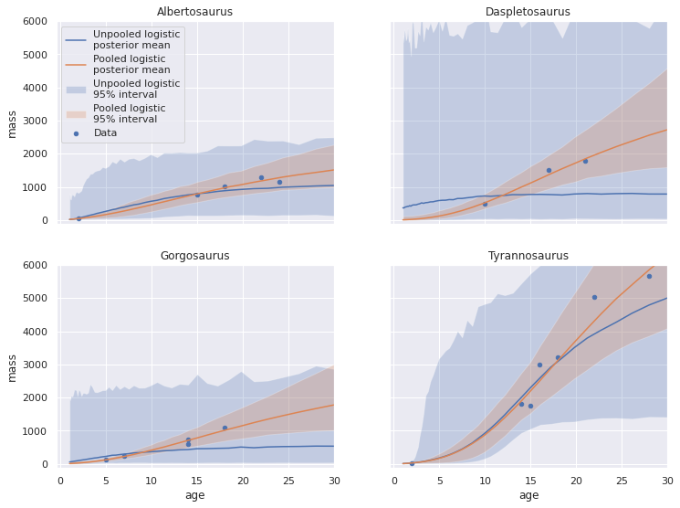
We see that the posterior predictive means for the pooled logistic model fit better than those from the unpooled model, and that the credible intervals are again significantly smaller.
We now compare the posterior predictions for the pooled log-linear and logistic models.
fig, axes = plot_pp_by_taxon(pp_pooled_loglin_df, plot_data=False, name="Pooled log-linear")
plot_pp_by_taxon(pp_pooled_logistic_df,
                 name="Pooled logistic",
                 fig=fig, axes=axes);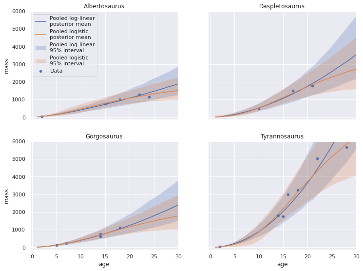
These models agree with each other fairly well, espescially in age ranges where the taxon data is concentrated, with the logistic model making slightly more plausible predictions as age increases.
Model comparison
We now compare these four models using two of the information criteria available in arviz. While BSM uses the deviance information criterion (DIC) to compare models, DIC is no longer supported in pymc3 or arviz, so we use Pareto-smoothed importance sampling leave-one-out cross validation (PSIS-LOO) and the widely applicable information criterion (WAIC) to compare models. These information criteria are available in arviz. For details on these methods, consult the pymc3 documentation.
traces = {
    'Unpooled log-linear': loglin_trace,
    'Pooled log-linear': pooled_loglin_trace,
    'Unpooled logistic': logistic_trace,
    'Pooled logistic': pooled_logistic_trace
}
def plot_compare(comp_df, ic, height=6, fig=None, axes=None):
if fig is None or axes is None:
fig, axes = plt.subplots(
ncols=2, figsize=(16 * (height / 6), height)
)
score_ax, weight_ax = axes
az.plot_compare(comp_df, insample_dev=False, plot_ic_diff=False, ax=score_ax)
score_ax.set_xlabel("Log score")
score_ax.set_ylabel("Model")
comp_df['weight'].plot.barh(ax=weight_ax)
weight_ax.set_xscale('log')
weight_ax.set_xlim(right=2)
weight_ax.set_xlabel("Stacking weight")
weight_ax.set_yticklabels([])
weight_ax.invert_yaxis()
fig.suptitle(f"{ic} comparison")
fig.tight_layout()
return fig, axesThe following plots show the PSIS-LOO comparison for these models.
loo_df = az.compare(traces, ic='loo', seed=SEED)
plot_compare(loo_df, "LOO");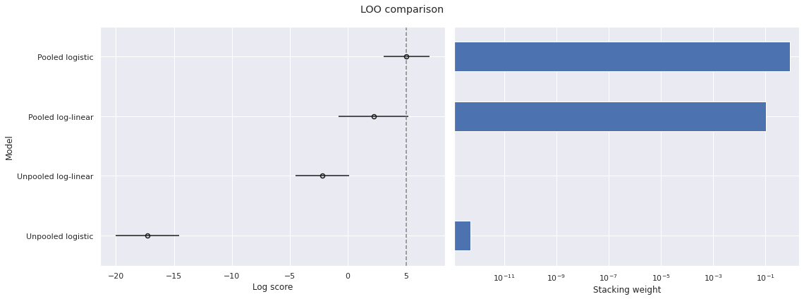
Note that larger scores are better, so PSIS-LOO favors the pooled models over the unpooled models and favors the pooled logistic model most highly of all.
waic_df = az.compare(traces, ic='waic', seed=SEED)
plot_compare(waic_df, "WAIC");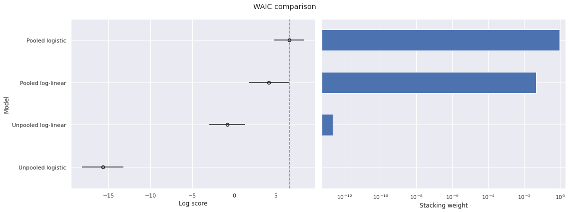
Using WAIC produces quite similar results.
Interestingly, the results in BSM using DIC favor the logistic model slightly.
Many thanks to Reich and Ghosh for their excellent textbook which brought this fun dataset to my attention and to Kiril Zvezdarov for his comments on early drafts.
The notebook this post was generated from is available here.
%load_ext watermark
%watermark -n -u -v -iv
Last updated: Sun May 16 2021
Python implementation: CPython
Python version : 3.8.8
IPython version : 7.22.0
pymc3 : 3.11.1
seaborn : 0.11.1
pandas : 1.2.3
arviz : 0.11.2
matplotlib: 3.4.1
numpy : 1.20.2
aesara : 2.0.6