Bayesian Factor Analysis Regression in Python with PyMC3

Wikipedia defines factor analysis as

a statistical method used to describe variability among observed, correlated variables in terms of a potentially lower number of unobserved variables called factors.

Factor analysis is used frequently in fields such as psychometrics, political science, and many others to identify latent (unmeasurable) traits that influence the observable behavior of people and systems.

Mathematically, Machine Learning: A Probabilistic Perspective (my favorite ML reference) describes factor analysis as “a low rank parametrization of [a multivariate normal distribution]” and as “a way of specifying a joint density model on [the vector] \(\mathbf{x}\)” using a small number of parameters.

This post will show how to add a richer covariance structure to the analysis of a simulated multivariate regression problem using factor analysis in Python with PyMC3. As we will see, specifying this model is somewhat tricky due to identifiability issues with naive model specifications.

Simulated data

We begin by simulating the data that we will subsequently analyze. First we make the necessary python imports and do some light housekeeping.

%matplotlib inline

from warnings import filterwarnings

from aesara import tensor as at
import arviz as az
from matplotlib import pyplot as plt
import numpy as np
import pymc3 as pm
import seaborn as sns

You are running the v4 development version of PyMC3 which currently still lacks key features. You probably want to use the stable v3 instead which you can either install via conda or find on the v3 GitHub branch: https://github.com/pymc-devs/pymc3/tree/v3

filterwarnings('ignore', category=RuntimeWarning, module='arviz')
filterwarnings('ignore', category=UserWarning, module='arviz')
filterwarnings('ignore', category=UserWarning, module='pandas')

plt.rcParams['figure.figsize'] = (8, 6)
sns.set(color_codes=True)

The observed predictors, \(\mathbf{x}_i\), will be \(5\)-dimensional vectors with entries drawn i.i.d. from the standard normal distribution. We generate 100 such vectors.

SEED = 123456789 # for reproducibility

rng = np.random.default_rng(SEED)

N = 100
K = 5

X = rng.normal(size=(N, K))

The observed targets, \(\mathbf{y}_i\), will be 10-dimensional vectors.

The constant term for this model, \(B_0\), is therefore a random vector in \(\mathbb{R}^{10}\) whose entries are i.i.d. drawn from the uniform distribution on \([-3, 3]\).

M = 10

B0 = rng.uniform(-3., 3., size=M)

The component slopes form a \(10 \times 5\) dimensional matrix. We generate a somewhat sparse matrix that has only (approximately) 50% of entries nonzero. These entries are also i.i.d. from the uniform distribution on \([-3, 3]\).

B = np.zeros((M, K))
P_nonzero = 0.5

is_nonzero = np.random.binomial(1, P_nonzero, size=(M, K)) == 1
B[is_nonzero] = rng.uniform(-3., 3., size=is_nonzero.sum())

The observations before noise are

\[\mathbf{y}_i^{\text{noiseless}} = B_0 + B\ \mathbf{x}_i.\]

Y_noiseless = B0 + X.dot(B.T)

So far this is a fairly standard simulation from a linear regression model. Things start to get more interesting when we introduce a non-diagonal correlation structure to the noise using latent factors. The noise added to the \(j\)-th component of the \(i\)-th sample is

\[\varepsilon_{i, j} = \mathbf{w}_j \cdot \mathbf{z}_i + \sigma_{i, j}\]

where \(\mathbf{w}_1, \cdots \mathbf{w}_{10}\), and \(\mathbf{z}_1, \ldots, \mathbf{z}_{100}\) are vectors in \(\mathbb{R}^2\) whose entries are drawn i.i.d. from a standard normal distribution. Here two is the number of latent factors that govern the covariance structure. The uncorrelated noise is drawn i.i.d. from a normal distribution with variance \((0.25)^2\).

F = 2

S_SCALE = 1.

W = rng.normal(size=(M, F))
Z = rng.normal(size=(N, F))

S = rng.normal(scale=S_SCALE, size=(N, M))

We now add this noise to our noiseless “data” to produce the actual observations.

Y = Y_noiseless + Z.dot(W.T) + S

Plotting the components of \(\mathbf{x}_i\) against those of \(\mathbf{y}_i\), we see (somewhat) sparse linear patterns emerge.

fig, axes = plt.subplots(nrows=M, ncols=K,
                         sharex=True, sharey=True,
                         figsize=(20, 12))

for j, row_axes in enumerate(axes):
    for i, ax in enumerate(row_axes):
        ax.scatter(X[:, i], Y[:, j], alpha=0.5);

        ax.set_xlabel(f"$x_{{{i + 1}}}$");
        ax.set_ylabel(f"$y_{{{j + 1}}}$");

fig.tight_layout();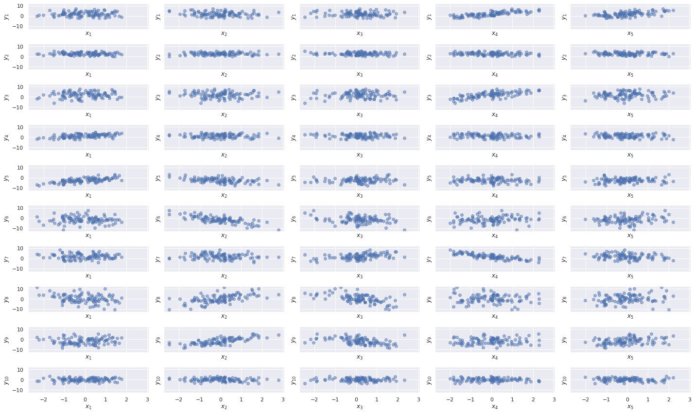

Modeling

We now begin building a series of models of this data using PyMC3.

No latent factors

We start with a simple multivariate regression model that assumes diagonal covariance to see the impact of ignoring the latent factors on our model.

We place i.i.d. \(N(0, 5^2)\) priors on the components of the intercepts (\(\beta_0\)) and the slopes (\(\beta\)).

with pm.Model() as multi_model:
    β0 = pm.Normal("β0", 0., 5., shape=M)
    β = pm.Normal("β", 0., 5., shape=(M, K))

The noise scale gets the prior \(\sigma \sim \text{Half}-N(2.5^2)\).

with multi_model:
    σ = pm.HalfNormal("σ", 2.5)

We now specify the likelihood of the observed data given the covariates.

with multi_model:
    μ = β0 + at.dot(X, β.T)
    obs = pm.Normal("obs", μ, σ, observed=Y)

We now sample from the posterior distribution of these parameters.

CORES = 4

SAMPLE_KWARGS = {
    'cores': CORES,
    'init': 'adapt_diag',
    'random_seed': [SEED + i for i in range(CORES)],
    'return_inferencedata': True
}

with multi_model:
    multi_trace = pm.sample(**SAMPLE_KWARGS)

Auto-assigning NUTS sampler...
Initializing NUTS using adapt_diag...
Multiprocess sampling (4 chains in 4 jobs)
NUTS: [β0, β, σ]

Sampling 4 chains for 1_000 tune and 1_000 draw iterations (4_000 + 4_000 draws total) took 56 seconds.

Standard sampling diagnostics (energy plots, BFMI, and \(\hat{R}\)) show no cause for concern.

def make_diagnostic_plots(trace, axes=None,
                          min_mult=0.995, max_mult=1.005,
                          var_names=None):
    if axes is None:
        fig, axes = plt.subplots(ncols=2,
                                 sharex=False, sharey=False,
                                 figsize=(16, 6))
        
    az.plot_energy(trace, ax=axes[0])
    
    
    rhat = az.rhat(trace, var_names=var_names).max()
    axes[1].barh(np.arange(len(rhat.variables)), rhat.to_array(),
                 tick_label=list(rhat.variables.keys()))
    axes[1].axvline(1, c='k', ls='--')

    axes[1].set_xlim(
        min_mult * min(rhat.min().to_array().min(), 1),
        max_mult * max(rhat.max().to_array().max(), 1)
    )
    axes[1].set_xlabel(r"$\hat{R}$")

    axes[1].set_ylabel("Variable")
    
    return fig, axes

make_diagnostic_plots(multi_trace);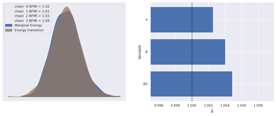

The following plot shows excellent agreement between the actual and estimated values of the intercepts.

ax, = az.plot_forest(multi_trace, var_names="β0", hdi_prob=0.95)

ax.scatter([], [],
           facecolors='none', edgecolors='C0',
           label="Posterior expected value");
ax.scatter(B0, ax.get_yticks()[::-1],
           c='k', zorder=5,
           label="Actual");

ax.set_yticklabels([]);
ax.set_ylabel(r"$\beta_0$");

ax.legend(loc="upper left");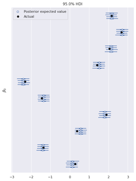

There is similarly excellent agreement for the component coefficients.

ax, = az.plot_forest(multi_trace, var_names="β",
                     coords={"β_dim_1": 0},
                     hdi_prob=0.95)

ax.scatter([], [],
           facecolors='none', edgecolors='C0',
           label="Posterior expected value");
ax.scatter(B[:, 0], ax.get_yticks()[::-1],
           c='k', zorder=5,
           label="Actual");

ax.set_yticklabels([]);
ax.set_ylabel(r"$\beta_{i, 0}$");

ax.legend(loc="upper left");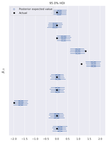

Note that here we have only plotted the posterior distributions for the first column of \(\beta\). The results are similar for the other columns.

az.plot_posterior(multi_trace, var_names="σ", ref_val=S_SCALE);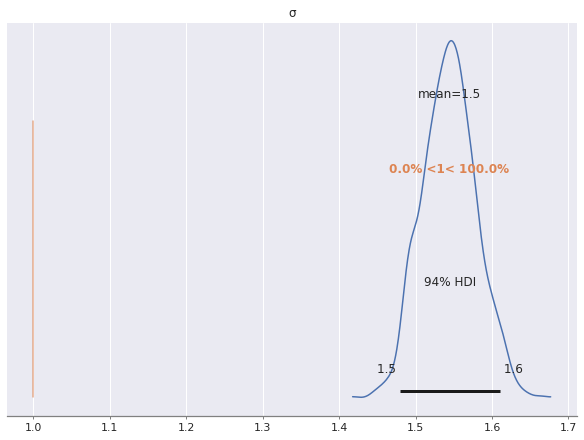

As we can see, the posterior estimate of \(\sigma\) is much higher than the true uncorrelated noise scale of one. This is due to the fact that we have not modeled the correlated noise induced by the latent factors. Indeed, since

\[\varepsilon_{i, j} = \mathbf{w}_j \cdot \mathbf{z}_i + \sigma_{i, j},\]

we get

\[ \begin{align*} \operatorname{Var}(\varepsilon_{i, j}) & = \operatorname{Var}(\mathbf{w}_j \cdot \mathbf{z}_i + \sigma_{i, j}) \\ & = 2 \operatorname{Var}(w_{i, j}) \cdot \operatorname{Var}(z_{i, j}) + 1^2 \\ & = 3, \end{align*} \]

since \(w_{i, j}\) and \(z_{i, j}\) are independent standard normal variables, which are also independent of \(\sigma_{i, j}\). Not accounting for the variation induced by the \(\mathbf{w}_j \cdot \mathbf{z}_i\) term in this model has caused the estimate of the scale of \(\sigma\) to be inflated.

With latent factors

We now add latent factors to our model, starting with the most straightforward parametrization. The priors on \(\beta_0\), \(\beta\), and \(\sigma\) are the same as for the previous model.

with pm.Model() as factor_model:
    β0 = pm.Normal("β0", 0., 5., shape=M)
    β = pm.Normal("β", 0., 5., shape=(M, K))
    μ = β0 + at.dot(X, β.T)
    
    σ = pm.HalfNormal("σ", 2.5)

We place i.i.d. standard normal priors on the entries of \(\mathbf{w}_j\) and \(\mathbf{z}_i\). and add their product to the expected value of observations.

with factor_model:
    w = pm.Normal("w", 0., 1., shape=(M, F))
    z = pm.Normal("z", 0., 1., shape=(N, F))
    
    obs = pm.Normal("obs", μ + z.dot(w.T), σ, observed=Y)

Again we sample from the posterior distribution of this model.

START_MULT = 3.

START_CORNERS = np.array([
    [1., 1.],
    [-1., 1.],
    [-1., -1.],
    [1., -1.]
])

w_starts = [
    {"w": w_start, "z": np.ones((N, F))} for w_start
        in START_MULT * np.ones((1, M, F)) * START_CORNERS[:, np.newaxis]
]

with factor_model:
    factor_trace = pm.sample(start=w_starts, **SAMPLE_KWARGS)

Auto-assigning NUTS sampler...
Initializing NUTS using adapt_diag...
Multiprocess sampling (4 chains in 4 jobs)
NUTS: [β0, β, σ, w, z]

Sampling 4 chains for 1_000 tune and 1_000 draw iterations (4_000 + 4_000 draws total) took 193 seconds.
The rhat statistic is larger than 1.4 for some parameters. The sampler did not converge.
The estimated number of effective samples is smaller than 200 for some parameters.

The \(\hat{R}\) statistics for \(\mathbf{z}_i\) and \(\mathbf{w}_j\) are quite high and warrant investigation.

make_diagnostic_plots(factor_trace);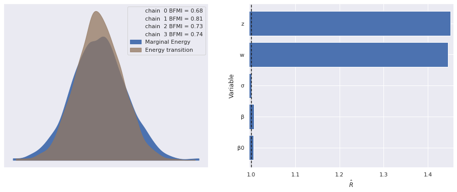

In spite of the large \(\hat{R}\) statistics, the estimate of the scale of \(\sigma\) is quite accurate for this model, since we have accounted for the noise due to the latent variables.

az.plot_posterior(factor_trace, var_names="σ", ref_val=S_SCALE);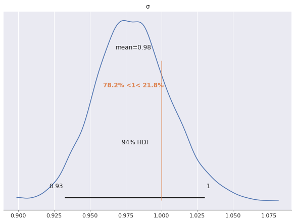

We turn to the posterior distributions of the factor loadings \(\mathbf{w}_j\). Below we plot the first two entries in \(\mathbf{w}_0\) and \(\mathbf{w}_1\) against each other.

ax = az.plot_pair(factor_trace, var_names="w",
                  coords={"w_dim_0": [0, 1], "w_dim_1": 0},
                  scatter_kwargs={'alpha': 0.5})

ax.set_xlabel("$w_{0, 0}$");
ax.set_ylabel("$w_{1, 0}$");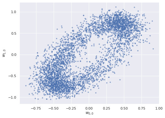

The elliptical shape of this posterior distribution is certainly unusual; let’s see what the pairwise plots look like for all pairs of entries in the factor loadings.

axes = az.plot_pair(factor_trace, var_names="w",
                   scatter_kwargs={'alpha': 0.5})

for ax in axes.flat:
    ax.set_xlabel(None);
    ax.set_ylabel(None);

axes[0, 0].figure.tight_layout();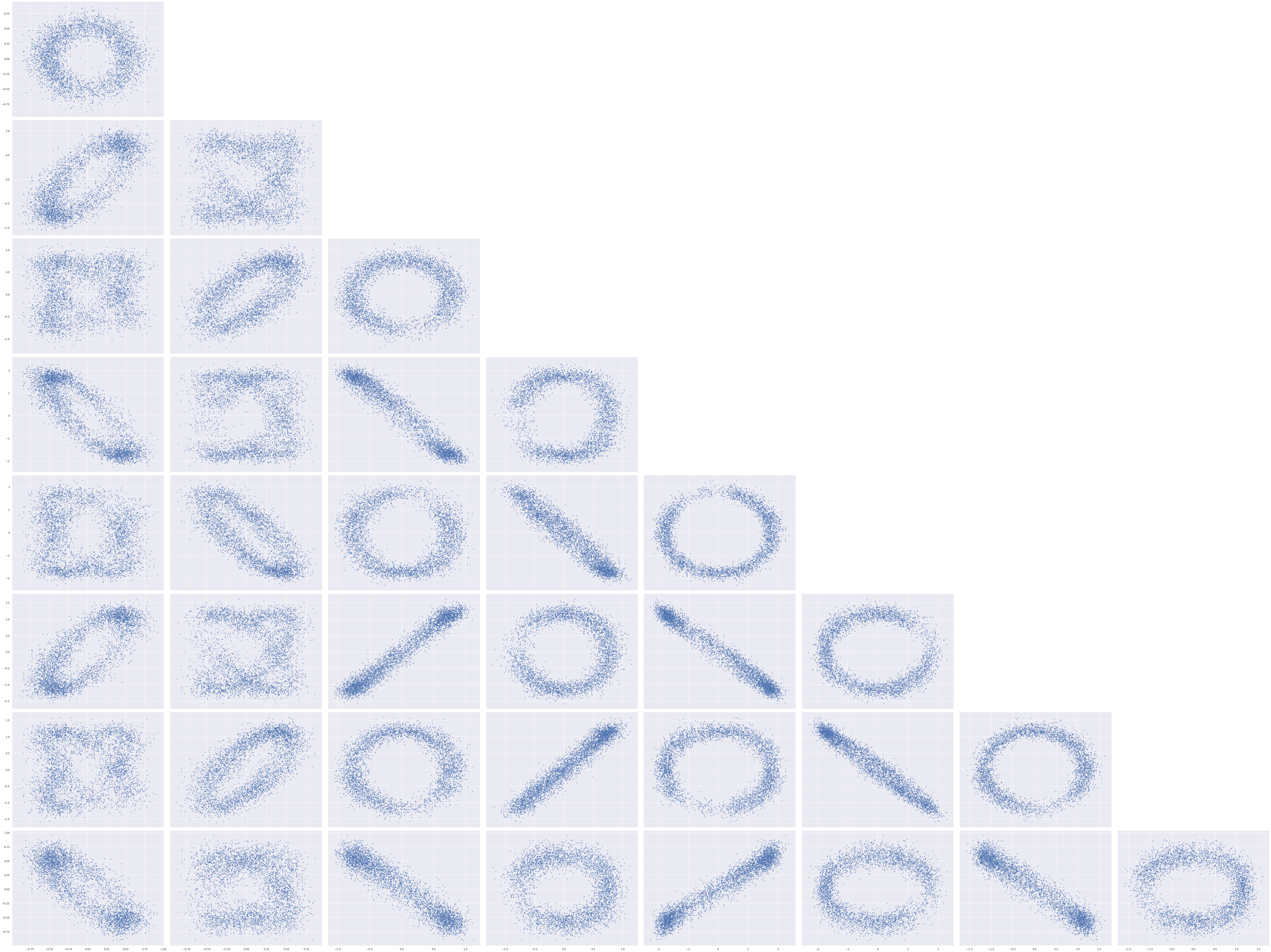

The shape of these posterior plots are odd indeed. These ellipses arise from the fact that the likelihood of the observed data is invariant under rotations of the latent two-dimensional space that the \(\mathbf{w}_j\)s live in.

To demonstrate this rotation invariance recall that

\[y_{i, j}\ |\ \mathbf{x}_i, \mathbf{w}_j, \mathbf{z}_i, \beta_0, \beta, \sigma \sim N\left(\beta_0 + \beta_j \cdot \mathbf{x}_i + \mathbf{w}_j \cdot \mathbf{z}_i, \sigma^2\right).\]

Let \(R \in \mathbb{R}^{2 \times 2}\) be a rotation matrix, so \(R^{\top} R = I_2\). Define \(\tilde{\mathbf{w}}_j = R \mathbf{w}_j\) and \(\tilde{\mathbf{z}}_i = R \mathbf{z}_i\), so

\[ \begin{align*} \tilde{\mathbf{w}}_j \cdot \tilde{\mathbf{z}}_i & = \tilde{\mathbf{w}}_j^{\top} \tilde{\mathbf{z}}_i \\ & = \mathbf{w}_j^{\top} R^{\top} R \mathbf{z}_i \\ & = \mathbf{w}_j^{\top} \mathbf{z}_i \\ & = \mathbf{w}_j \cdot \mathbf{z}_i. \end{align*} \]

Because rotation by \(R\) preserves dot products, \(y_{i, j}\ |\ \mathbf{x}_i, \mathbf{w}_j, \mathbf{z}_i, \beta_0, \beta, \sigma\) and \(y_{i, j}\ |\ \mathbf{x}_i, \tilde{\mathbf{w}}_j, \tilde{\mathbf{z}}_i, \beta_0, \beta, \sigma\) have the same distribution.

Breaking rotation invariance

There are a number of ways to deal with the rotational invariance of this model’s naively parametrized likelihood. Those interested in maximum likelihood (MLE) or regularized maximum likelihood (maxium a priori/MAP) estimation usually don’t worry about rotational invariance as all rotations should produce the same likelihood. In this case practitioners may use whichever solution their gradient descent algorithm converges to, or they may choose an informative rotation based on their application. In Bayesian MCMC estimation, sometimes the non-identification is embraced and a rotation is fixed after sampling. I tend to find such approaches unsatisfying, as they render our convergence checks less useful than they are for a fully identified model.

Fortunately a paper of Peeters¹ gives sufficient conditions for priors on \(\mathbf{w}_j\) to break this rotational symmetry. With \(N\) observations, let

\[ \begin{align*} W & = \begin{pmatrix} \mathbf{w}_1 \\ \vdots \\ \mathbf{w}_N \end{pmatrix} \end{align*} \]

be the matrix with the loading factors as its rows. For factors of latent dimension \(F\), Peeter’s conditions are

1. \(W\) has at least \(F - 1\) fixed zero entries in each column.
2. For each column, the rank of the of the submatrix that results from deleting the rows where that column has fixed zeros should be \(M - 1\).
3. The covariance matrix of the \(\mathbf{z}_i\)s is one on the diagonal.
4. At least one value in each column is constrained to either be positive or negative only.

Conditions 1, 3, and 4 are easy enough to satisfy as we will see. After a bit of reflection, condition 2 is also almost always satisfied for the following technical reason. Assume the matrix, \(X\), is square of dimension \(N \times N\) and not invertible. We must have \(\operatorname{det} X = 0\), which means that the set of invertible matrices form an \(N^2 - 1\) dimensional manifold in the \(N^2\) dimensional space \(\mathbb{R}^{N \times N}\). Since every set of less than full dimension has Lebesgue measure zero, as long as we choose a random matrix from a reasonable distribution (one that is absolutely continuous with respect to the Lebesgue measure) it will almost certainly not have determinant zero and therefore have full rank. More technical arguments show that this is also true of non-square matrices drawn from reasonable distributions.

We now build a new representation of this model that satisfies these four conditions for breaking rotational invariance. The priors on \(\beta_0\), \(\beta\), \(\sigma\), and \(\mathbf{z}_i\) are the same as for the previous model.

with pm.Model() as rot_model:
    β0 = pm.Normal("β0", 0., 5., shape=M)
    β = pm.Normal("β", 0., 5., shape=(M, K))
    μ = β0 + at.dot(X, β.T)
    
    σ = pm.HalfNormal("σ", 2.5)
    
    z = pm.Normal("z", 0., 1., shape=(N, F))

For our two-dimensional example, we will build a factor loading matrix, \(W\), of the following form in stages.

\[ W = \begin{pmatrix} 1 & 0 \\ 0 & 1 \\ + & + \\ ? & ? \\ \vdots & \vdots \\ ? & ? \end{pmatrix} \]

Here \(+\) means that the entry is constrained to be positive and \(?\) means that entry is unconstrained. First we set the first two rows to be the two-by-two identity matrix.

w_top = at.eye(M, F)

Next we add the row of entries constrained to be positive below that.

HALFNORMAL_SCALE = 1. / np.sqrt(1. - 2. / np.pi)

with rot_model:
    w_top_pos = at.set_subtensor(
        w_top[F],
        pm.HalfNormal("w_pos", HALFNORMAL_SCALE, shape=F)
    )

Note that HALFNORMAL_SCALE is the scale necessary for the entries in this row to have variance one.

Finally, we add the bottom block of unconstrained entries.

with rot_model:
    w = pm.Deterministic("w", at.set_subtensor(
        w_top_pos[F + 1:],
        pm.Normal("w_block", 0., 1., shape=(M - (F + 1), F))
    ))

Evaluating w shows that it has the desired structure.

w.eval()

array([[ 1.        ,  0.        ],
       [ 0.        ,  1.        ],
       [ 1.20384406,  4.14310473],
       [-0.14646375, -0.84303061],
       [ 1.10983887,  0.49052328],
       [-1.89554466,  0.67558106],
       [-0.96375033,  0.02590003],
       [-0.10067908,  0.25301074],
       [-0.97963568, -1.44020378],
       [-0.48985021,  0.40814108]])

The likelihood of the observed data is the same as in the previous model.

with rot_model:
    obs = pm.Normal("obs", μ + z.dot(w.T), σ, observed=Y)

Again we sample from the posterior distribution of this model.

w_block_starts = [
    {"w_block": w_start, "z": np.ones((N, F))} for w_start
        in START_MULT * np.ones((1, M - (F + 1), F)) * START_CORNERS[:, np.newaxis]
]

with rot_model:
    rot_trace = pm.sample(start=w_block_starts, **SAMPLE_KWARGS)

Auto-assigning NUTS sampler...
Initializing NUTS using adapt_diag...
Multiprocess sampling (4 chains in 4 jobs)
NUTS: [β0, β, σ, z, w_pos, w_block]

Sampling 4 chains for 1_000 tune and 1_000 draw iterations (4_000 + 4_000 draws total) took 176 seconds.
There were 320 divergences after tuning. Increase `target_accept` or reparameterize.
The acceptance probability does not match the target. It is 0.5597958935132601, but should be close to 0.8. Try to increase the number of tuning steps.
The rhat statistic is larger than 1.4 for some parameters. The sampler did not converge.
The estimated number of effective samples is smaller than 200 for some parameters.

The marginal energy plot is bimodal, which is quite unusual, and the \(\hat{R}\) statistics are still quite high.

make_diagnostic_plots(rot_trace);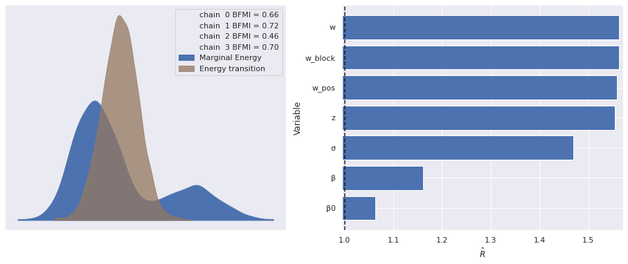

To diagnose these issues, we investigate the posterior distributions of these noise parameters.

The posterior distribution of \(\sigma\) appears to be bimodal, with one local maximum twice as high as the other. This would seem to indicate that two of our three chains spent their time in the mode corresponding two smaller values of \(\sigma\) and the other chain spent its time in the mode corresponding to the higher value of \(\sigma\).

az.plot_posterior(rot_trace, var_names="σ", ref_val=S_SCALE);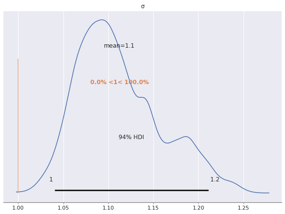

Sure enough, plotting the trace of each chain confirms this suspiscion.

az.plot_trace(rot_trace, var_names="σ");

The pair plots for the unconstrained entries of w_block show that we have successfully broken the rotational invariance of the naive factor model, but also show bimodal behavior.

axes = az.plot_pair(rot_trace, var_names="w_block",
                   scatter_kwargs={'alpha': 0.5})

for ax in axes.flat:
    ax.set_xlabel(None);
    ax.set_ylabel(None);

axes[0, 0].figure.tight_layout();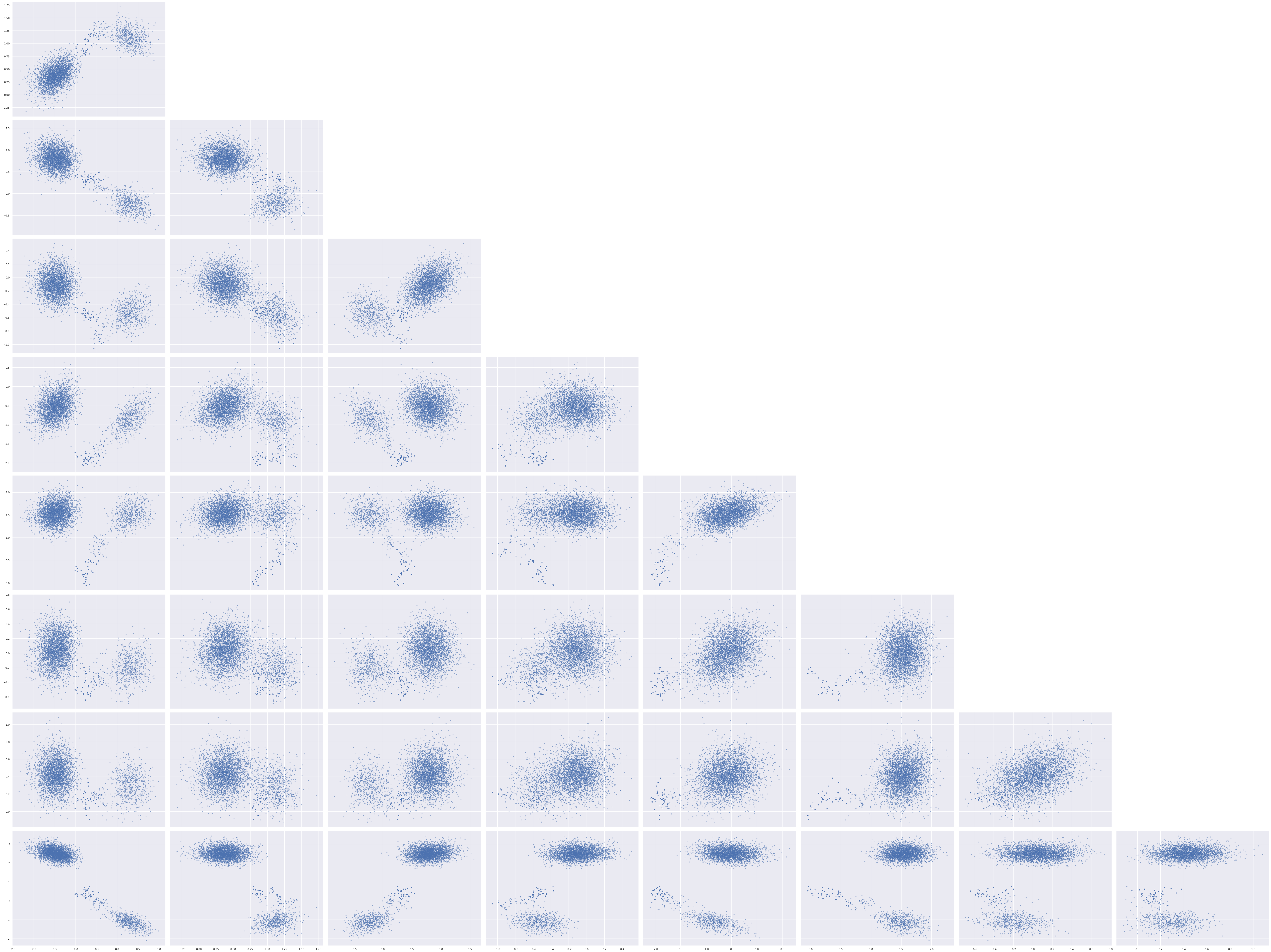

We see here that even though we appear to have broken the rotation invariance of the likelihood, it remains unidentified in the case that the signs of the \(\mathbf{w}_j\)s and \(\mathbf{z}_i\)s are changed in a consistent manner. To see this invariance, notice that if \(R \in \mathbb{R}^{2 \times 2}\) is diagonal with nonzero entries in the set \(\{-1, 1\}\), then \(R^{\top} R = I_2\) and the previous algebra shows that the likelihood is invariant under transformation of the latent parameters by \(R\).

Breaking reflection invariance

To break this reflection invariance, we fix the signs on one of the unconstrained factor loadings, \(\mathbf{w}_j\) and preserve the relationship between its signs and the signs of the corresponding entries of the other \(\mathbf{w}_j\)s and \(\mathbf{z}_i\)s. We choose to fix the sign of the factor loading that has the largest \(\hat{R}\) statistic in one of its columns, as this will be the loading with the most extreme reflection symmetry. We denote this loading’s index by \(\hat{j}\).

j_hat, = (az.rhat(rot_trace, var_names="w_block")
            .max(dim="w_block_dim_1")
            .argmax(dim="w_block_dim_0")
            .to_array()
            .data)

ax = az.plot_pair(rot_trace, var_names="w_block",
                  coords={"w_block_dim_0": j_hat},
                  scatter_kwargs={'alpha': 0.25})

ax.set_xlabel("");
ax.set_ylabel("");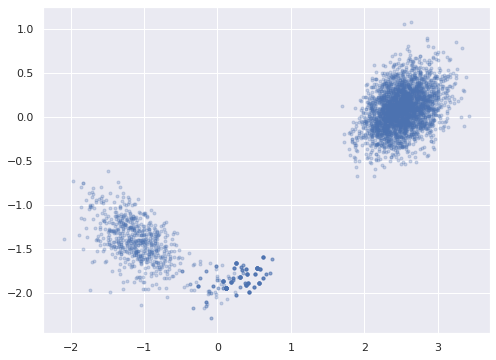

We choose the target signs of the entries in \(\mathbf{w}_{\hat{j}}\).

target_sign = np.sign(
    rot_trace["posterior"]["w_block"]
             [0, :, j_hat]
             .mean(dim="draw")
             .data
)

The priors on \(\beta_0\), \(\beta\), \(\sigma\), are the same as for the previous model, as is most of the construction of \(\mathbf{w}_j\) and \(\mathbf{z}_i\).

with pm.Model() as ref_model:
    β0 = pm.Normal("β0", 0., 5., shape=M)
    β = pm.Normal("β", 0., 5., shape=(M, K))
    μ = β0 + at.dot(X, β.T)
    
    σ = pm.HalfNormal("σ", 2.5)

w_top = at.eye(M, F)

with ref_model:
    w_top_pos = at.set_subtensor(
        w_top[F],
        pm.HalfNormal("w_pos", HALFNORMAL_SCALE, shape=F)
    )
    w_block_ = pm.Normal("w_block_", 0., 1., shape=(M - (F + 1), F))

We now enforce our choice of signs on \(\mathbf{w}_j\) and \(\mathbf{z}_i\).

with ref_model:
    w_block = pm.Deterministic(
        "w_block",
        target_sign * at.sgn(w_block_[j_hat]) * w_block_
    )
    w = pm.Deterministic("w", at.set_subtensor(
        w_top_pos[F + 1:], w_block    
    ))

with ref_model:
    z_ = pm.Normal("z_", 0., 1., shape=(N, F))
    z = pm.Deterministic(
        "z", target_sign * at.sgn(w_block_[j_hat]) * z_
    )

The likelihood of the observed data is the same as in the previous model.

with ref_model:
    obs = pm.Normal("obs", μ + z.dot(w.T), σ, observed=Y)

Again we sample from the posterior distribution of this model.

with ref_model:
    ref_trace = pm.sample(**SAMPLE_KWARGS)

Auto-assigning NUTS sampler...
Initializing NUTS using adapt_diag...
Multiprocess sampling (4 chains in 4 jobs)
NUTS: [β0, β, σ, w_pos, w_block_, z_]

Sampling 4 chains for 1_000 tune and 1_000 draw iterations (4_000 + 4_000 draws total) took 278 seconds.
There were 16 divergences after tuning. Increase `target_accept` or reparameterize.
The rhat statistic is larger than 1.4 for some parameters. The sampler did not converge.
The estimated number of effective samples is smaller than 200 for some parameters.

The marginal energy plot plot looks much better for this model, as do the \(\hat{R}\) statistics. Note that here we have ignored the warnings about (and not plotted) the \(\hat{R}\) statistics for the untransformed w_block_ and z_, which we expect to be large, as they still are invariant under reflections.

rhat_var_names = [
    var_name for var_name in ref_trace["posterior"].data_vars
        if not var_name.endswith("_")
]
make_diagnostic_plots(ref_trace, var_names=rhat_var_names);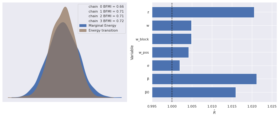

Plotting the posterior distribution of \(w_{4, 0}\), we can see that we have in fact broken reflection invariance and fully identified our model.

ax = az.plot_pair(ref_trace, var_names="w_block",
                  coords={"w_block_dim_0": j_hat},
                  scatter_kwargs={'alpha': 0.25})


ax.set_xlabel("");
ax.set_ylabel("");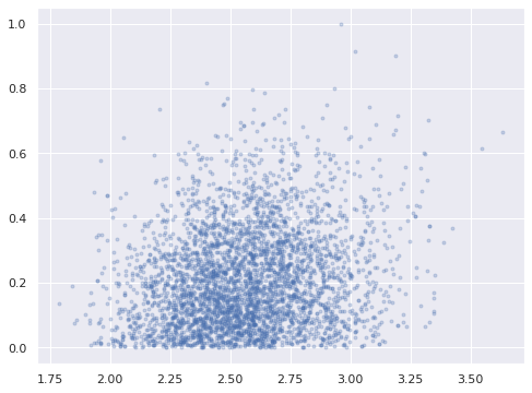

In this fully identified model, the posterior expected value of the parameters shows good agreements with the true values used to generate the data.

ax, = az.plot_forest(ref_trace, var_names="β0", hdi_prob=0.95)

ax.scatter([], [],
           facecolors='none', edgecolors='C0',
           label="Posterior expected value");
ax.scatter(B0, ax.get_yticks()[::-1],
           c='k', zorder=5,
           label="Actual");

ax.set_yticklabels([]);
ax.set_ylabel(r"$\beta_0$");

ax.legend(loc="upper left");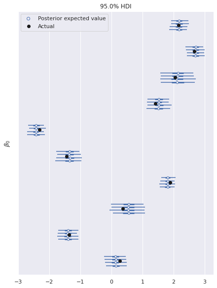

ax, = az.plot_forest(ref_trace, var_names="β",
                     coords={"β_dim_1": 0},
                     hdi_prob=0.95)

ax.scatter([], [],
           facecolors='none', edgecolors='C0',
           label="Posterior expected value");
ax.scatter(B[:, 0], ax.get_yticks()[::-1],
           c='k', zorder=5,
           label="Actual");

ax.set_yticklabels([]);
ax.set_ylabel(r"$\beta_{i, 0}$");

ax.legend(loc="upper left");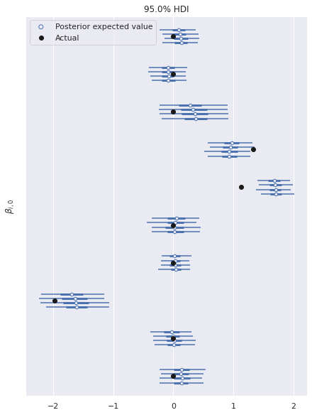

az.plot_posterior(ref_trace, var_names="σ", ref_val=S_SCALE);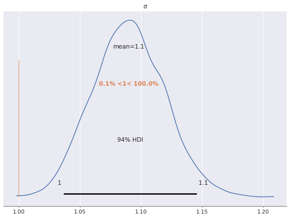

Note that with more latent dimensions we would need to constrain the signs of more factor loadings to completely break reflection invariance.

This post is available as a Jupyter notebook here.

%load_ext watermark
%watermark -n -u -v -iv

Last updated: Mon Jul 05 2021

Python implementation: CPython
Python version       : 3.8.8
IPython version      : 7.22.0

arviz     : 0.11.2
pymc3     : 4.0
numpy     : 1.20.2
aesara    : 2.0.12
matplotlib: 3.4.1
seaborn   : 0.11.1