A Fair Price for the Republic Gunship? A Bayesian Analysis of Ultimate Collector Series Prices in Python with PyMC3

Austin Rochford

2021-07-20

Since my last post on modeling Lego prices, Lego has announced the release of 73509, an Ultimate Collector Series Republic Gunship from the Battle of Geonosis.

As with 75296, Darth Vader Meditation Chamber, we can ask whether the $349.99 recommended retail price of this set is fair given its number of pieces, Star Wars theme, and Ultimate Collector Series status. This post will update the model from the previous one to include random effects for subtheme (in Lego collector jargon, the theme of 75309 is “Star Wars” and the subtheme is “Ultimate Collector Series”) to answer this question. In addition, we will explore the effect of different themes and subthemes on set prices.

First we make some Python imports and do a bit of housekeeping.

%matplotlib inline

import datetime
from functools import reduce
from warnings import filterwarnings

from aesara import shared, tensor as at
import arviz as az
from matplotlib import MatplotlibDeprecationWarning, pyplot as plt
from matplotlib.ticker import StrMethodFormatter
import numpy as np
import pandas as pd
import pymc3 as pm
from sklearn.preprocessing import StandardScaler
import seaborn as sns

You are running the v4 development version of PyMC3 which currently still lacks key features. You probably want to use the stable v3 instead which you can either install via conda or find on the v3 GitHub branch: https://github.com/pymc-devs/pymc3/tree/v3

filterwarnings('ignore', category=MatplotlibDeprecationWarning, module='pandas')
filterwarnings('ignore', category=UserWarning, module='aesara')
filterwarnings('ignore', category=UserWarning, module='arviz')
filterwarnings('ignore', category=UserWarning, module='pandas')

FIGSIZE = (8, 6)

plt.rcParams['figure.figsize'] = FIGSIZE
sns.set(color_codes=True)

dollar_formatter = StrMethodFormatter("${x:,.2f}")

Load the Data

We begin the real work by loading the data scraped from Brickset. See the first post in this series for more background on the data.

DATA_URL = 'https://austinrochford.com/resources/lego/brickset_01011980_06012021.csv.gz'

def to_datetime(year):
    return np.datetime64(f"{round(year)}-01-01")

full_df = (pd.read_csv(DATA_URL,
                       usecols=[
                           "Year released", "Set number",
                           "Name", "Set type", "Theme", "Subtheme",
                           "Pieces", "RRP"
                       ])
             .dropna(subset=[
                 "Year released", "Set number",
                 "Name", "Set type", "Theme",
                 "Pieces", "RRP"
             ]))
full_df["Year released"] = full_df["Year released"].apply(to_datetime)
full_df = (full_df.set_index(["Year released", "Set number"])
                  .sort_index())

We see that the data set contains information on approximately 8,500 Lego sets produced between 1980 and June 2021.

full_df.head()

		Name	Set type	Theme	Pieces	RRP	Subtheme
Year released	Set number
1980-01-01	1041-2	Educational Duplo Building Set	Normal	Dacta	68.0	36.50	NaN
	1075-1	LEGO People Supplementary Set	Normal	Dacta	304.0	14.50	NaN
	1101-1	Replacement 4.5V Motor	Normal	Service Packs	1.0	5.65	NaN
	1123-1	Ball and Socket Couplings & One Articulated Joint	Normal	Service Packs	8.0	16.00	NaN
	1130-1	Plastic Folder for Building Instructions	Normal	Service Packs	1.0	14.00	NaN

full_df.tail()

		Name	Set type	Theme	Pieces	RRP	Subtheme
Year released	Set number
2021-01-01	80022-1	Spider Queen’s Arachnoid Base	Normal	Monkie Kid	1170.0	119.99	Season 2
	80023-1	Monkie Kid’s Team Dronecopter	Normal	Monkie Kid	1462.0	149.99	Season 2
	80024-1	The Legendary Flower Fruit Mountain	Normal	Monkie Kid	1949.0	169.99	Season 2
	80106-1	Story of Nian	Normal	Seasonal	1067.0	79.99	Chinese Traditional Festivals
	80107-1	Spring Lantern Festival	Normal	Seasonal	1793.0	119.99	Chinese Traditional Festivals

full_df.describe()

	Pieces	RRP
count	8502.000000	8502.000000
mean	258.739591	31.230506
std	481.627846	44.993559
min	0.000000	0.000000
25%	32.000000	7.000000
50%	98.000000	17.000000
75%	300.000000	39.990000
max	11695.000000	799.990000

CPI_URL = 'https://austinrochford.com/resources/lego/CPIAUCNS202100401.csv'

years = pd.date_range('1979-01-01', '2021-01-01', freq='Y') \
        + datetime.timedelta(days=1)
cpi_df = (pd.read_csv(CPI_URL, index_col="DATE", parse_dates=["DATE"])
        .loc[years])
cpi_df["to2021"] = cpi_df.loc["2021-01-01"] / cpi_df

We now add a column RRP2021, which is RRP adjusted to 2021 dollars.

full_df["RRP2021"] = (pd.merge(full_df, cpi_df,
                           left_on=["Year released"],
                           right_index=True)
                    .apply(lambda df: df["RRP"] * df["to2021"],
                           axis=1))

Based on the exploratory data analysis in the first post in this series, we filter full_df down to approximately 6,300 sets to be included in our analysis.

FILTERS = [
full_df["Set type"] == "Normal",
full_df["Pieces"] > 10,
full_df["Theme"] != "Duplo",
full_df["Theme"] != "Service Packs",
full_df["Theme"] != "Bulk Bricks",
full_df["RRP"] > 0
]

df = full_df[reduce(np.logical_and, FILTERS)].copy()

df.head()

		Name	Set type	Theme	Pieces	RRP	Subtheme	RRP2021
Year released	Set number
1980-01-01	1041-2	Educational Duplo Building Set	Normal	Dacta	68.0	36.50	NaN	122.721632
	1075-1	LEGO People Supplementary Set	Normal	Dacta	304.0	14.50	NaN	48.752429
	5233-1	Bedroom	Normal	Homemaker	26.0	4.50	NaN	15.130064
	6305-1	Trees and Flowers	Normal	Town	12.0	3.75	Accessories	12.608387
	6306-1	Road Signs	Normal	Town	12.0	2.50	Accessories	8.405591

df.describe()

	Pieces	RRP	RRP2021
count	6312.000000	6312.000000	6312.000000
mean	337.177440	37.038246	45.795998
std	535.619271	49.657704	58.952563
min	11.000000	0.600000	0.971220
25%	68.000000	9.990000	11.866173
50%	177.000000	19.990000	26.712319
75%	400.000000	49.500000	55.952471
max	11695.000000	799.990000	897.373477

Exploratory Data Analysis

The first post in this series does quite a lot of exploratory data analysis (EDA) on this data which we will not repeat here. For this post our EDA will focus on subtheme.

We see that there are a bit less than 500 subthemes and that just under a quarter of sets have no subtheme associated with them on Brickset.

df["Subtheme"].describe()

count       4896
unique       482
top       3 in 1
freq         189
Name: Subtheme, dtype: object

df["Subtheme"].isnull().mean()

0.22433460076045628

We see that there are many Technic sets with no subtheme, and a few other themes also stand out for having many sets with no subtheme.

ax = (df[df["Subtheme"].isnull()]
        ["Theme"]
        .value_counts()
        .plot.barh(figsize=(8, 16)))

ax.set_xscale('log');
ax.set_xlabel("Number of sets with no subtheme");

ax.invert_yaxis();
ax.set_ylabel("Theme");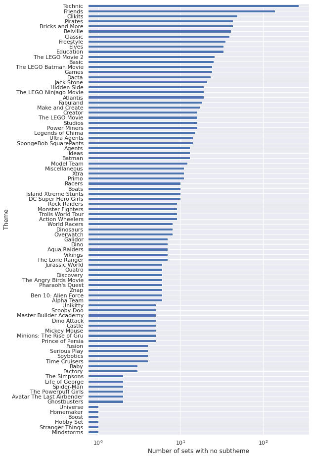

When we introduce subtheme-based random effects we will treat these sets with null subtheme values carefully.

Now we check whether or not each subtheme is only ever paired with one theme.

sub_n_themes = (df.groupby("Subtheme")
                  ["Theme"]
                  .nunique())

ax = (sub_n_themes.value_counts()
                  .plot.bar(rot=0))

ax.set_xlabel(("Number of themes associated\n"
               "with the subtheme"));

ax.set_yscale('log');
ax.set_ylabel("Number of subthemes");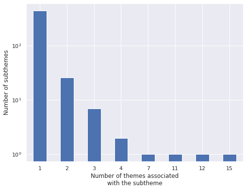

(sub_n_themes == 1).mean()

0.9190871369294605

This plot and calculation show that the vast majority (about 92%) of subthemes are associated with only one theme. We now examine the subthemes that are associated with more than one theme.

ax = (sub_n_themes[sub_n_themes > 1]
                  .sort_values()
                  .plot.barh(figsize=(8, 9)))

ax.set_xlabel(("Number of themes associated\n"
               "with the subtheme"));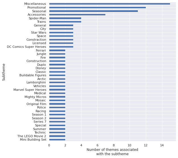

The subthemes associated with the most themes make sense, many themes will have “Miscellaneous,” “Promotional,” “Seasonal,” and “Accessories” sets. Of the remaining such subthemes, I personally am curious about the themes that the “Star Wars” subtheme is associated with.

STAR_WARS = "Star Wars"

ax = (df[df["Subtheme"] == STAR_WARS]
        ["Theme"]
        .value_counts()
        .plot.barh())

ax.set_xlabel(("Number of sets with\n"
               "\"Star Wars\" subtheme"))

ax.invert_yaxis();
ax.set_ylabel("Theme");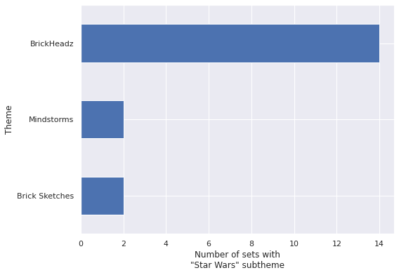

These themes make sense, there are “BrickHeadz” of many sorts (in addition to Star Wars, Disney, Harry Potter, and Pets come to mind immediately) and the same reasoning applies to “Brick Sketches” and “Mindstorms.”

In order to truly remain faithful to the source data, we will treat theme and subtheme as if they are not nested, even though in reality they are.

Modeling

Time-varying intercepts, theme-based random effects and slopes

We begin by rebuilding the final model from the previous post, which models the relationship between log RRP in 2021 dollars and log piece count using time-varying intercepts and time-constant slopes with theme-based random effects. For full details of this model please consult the previous post.

First we build the feature vector $x$ (standardized log price) and the target vector $y$ (log RRP in 2021 dollars).

pieces = df["Pieces"].values
log_pieces = np.log(df["Pieces"].values)

rrp2021 = df["RRP2021"].values
log_rrp2021 = np.log(rrp2021)

scaler = StandardScaler().fit(log_pieces[:, np.newaxis])

def scale_log_pieces(log_pieces, scaler=scaler):
    return scaler.transform(log_pieces[:, np.newaxis])[:, 0]

std_log_pieces = scale_log_pieces(log_pieces)
std_log_pieces_ = shared(std_log_pieces)

We also encode the themes as integer indices and calculate the (standardize) mean log piece count per theme in order to make an adjustment to satisfy the Gauss-Markov criteria.

theme_id, theme_map = df["Theme"].factorize(sort=True)
n_theme = theme_map.size

theme_id_ = shared(theme_id)

theme_mean_std_log_pieces = (pd.Series(std_log_pieces, index=df.index)
                               .groupby(df["Theme"])
                               .mean())

Finally we encode the year (in years since 1960) that the set was released for the time-varying component of the intercept.

year = df.index.get_level_values("Year released").year.values
t = year - year.min()
n_year = int(t.max() + 1)

t_ = shared(t)

We now define the final model of the previous post in PyMC3.

def hierarchical_normal(name, shape, μ=None):
    if μ is None:
        μ = pm.Normal(f"μ_{name}", 0., 2.5)

    Δ = pm.Normal(f"Δ_{name}", 0., 1., shape=shape)
    σ = pm.HalfNormal(f"σ_{name}", 2.5)
    
    return pm.Deterministic(name, μ + Δ * σ)

def hierarchical_normal_with_mean(name, x_mean, shape,
                                  μ=None, mean_name="γ"):
    mean_coef = pm.Normal(f"{mean_name}_{name}", 0., 2.5)
        
    return pm.Deterministic(
        name,
        hierarchical_normal(f"_{name}", shape, μ=μ) \
            + mean_coef * x_mean
    )

def gaussian_random_walk(name, shape, innov_scale=1.):
    Δ = pm.Normal(f"Δ_{name}", 0., innov_scale,  shape=shape)

    return pm.Deterministic(name, Δ.cumsum())

with pm.Model() as model:
    β0_0 = pm.Normal("β0_0", 0., 2.5)
    
    β0_t = gaussian_random_walk("β0_t", n_year, innov_scale=0.1)
    
    β0_theme = hierarchical_normal_with_mean(
        "β0_theme",
        at.constant(theme_mean_std_log_pieces),
        n_theme, μ=0.
    )
    β0_i = β0_0 + β0_t[t_] + β0_theme[theme_id_]

    
    β_pieces_0 = pm.Normal("β_pieces_0", 0., 2.5)
    
    β_pieces_theme = hierarchical_normal_with_mean(
        "β_pieces_theme",
        at.constant(theme_mean_std_log_pieces),
        n_theme, μ=0.
    )
    
    β_pieces = β_pieces_0 + β_pieces_theme
    
    σ = pm.HalfNormal("σ", 5.)
    μ = β0_i + β_pieces_theme[theme_id_] * std_log_pieces_ - 0.5 * σ**2
    
    obs = pm.Normal("obs", μ, σ, observed=log_rrp2021)

We are finally ready to sample from the posterior distribution of this model given the Brickset data.

CHAINS = 3
SEED = 123456789

SAMPLE_KWARGS = {
    'cores': CHAINS,
    'random_seed': [SEED + i for i in range(CHAINS)],
    'return_inferencedata': True
}

with model:
    trace = pm.sample(**SAMPLE_KWARGS)

Auto-assigning NUTS sampler...
Initializing NUTS using jitter+adapt_diag...
Multiprocess sampling (3 chains in 3 jobs)
NUTS: [β0_0, Δ_β0_t, γ_β0_theme, Δ__β0_theme, σ__β0_theme, β_pieces_0, γ_β_pieces_theme, Δ__β_pieces_theme, σ__β_pieces_theme, σ]

100.00% [6000/6000 09:51<00:00 Sampling 3 chains, 0 divergences]

Sampling 3 chains for 1_000 tune and 1_000 draw iterations (3_000 + 3_000 draws total) took 592 seconds.
The estimated number of effective samples is smaller than 200 for some parameters.

The standard sampling diagnostics show no cause for concern.

def plot_diagnostics(trace, axes=None, min_mult=0.995, max_mult=1.005):
    if axes is None:
        fig, axes = plt.subplots(ncols=2, sharex=False, sharey=False,
                                 figsize=(16, 6))
        
    az.plot_energy(trace, ax=axes[0])
    
    
    rhat = az.rhat(trace).max()
    axes[1].barh(np.arange(len(rhat.variables)), rhat.to_array(),
                 tick_label=list(rhat.variables.keys()))
    axes[1].axvline(1, c='k', ls='--')

    axes[1].set_xlim(
        min_mult * min(rhat.min().to_array().min(), 1),
        max_mult * max(rhat.max().to_array().max(), 1)
    )
    axes[1].set_xlabel(r"$\hat{R}$")

    axes[1].set_ylabel("Variable")
    
    return fig, axes

plot_diagnostics(trace);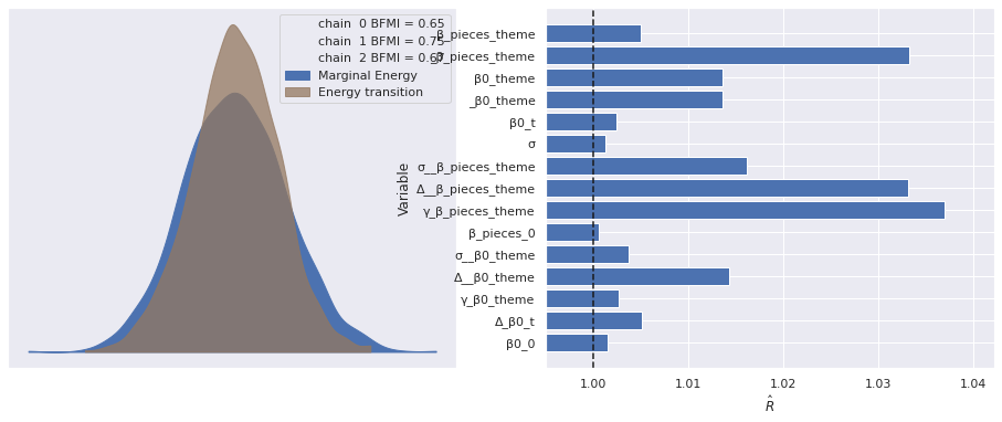

We now sample from the posterior predictive distribution of the model and visualize the resulting residuals.

with model:
    pp_data = pm.sample_posterior_predictive(trace)

df["pred"] = pp_data["obs"].mean(axis=0)
df["resid"] = log_rrp2021 - df["pred"]

100.00% [3000/3000 00:01<00:00]

ax = sns.scatterplot(x="Pieces", y="resid",
                     data=df.reset_index(),
                     color='C0', alpha=0.1);
(df.groupby(df["Pieces"].round(-2))
   ["resid"]
   .mean()
   .plot(c='k', label="Bucketed average",
         ax=ax));

ax.set_xscale('log');

ax.set_ylim(-2, 2);
ax.set_ylabel("Log RRP residual (2021 $)");

ax.legend(loc='upper left');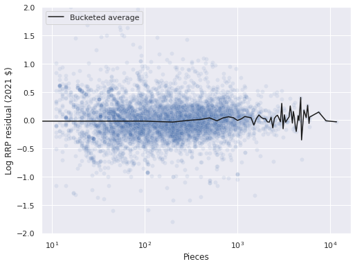

ax = (df.groupby(level="Year released")
        ["resid"]
        .mean()
        .plot(c='k', label="Year average"));

strip_ax = ax.twiny()
sns.stripplot(x="Year released", y="resid",
              data=df.reset_index(),
              jitter=1.5,
              color='C0', alpha=0.1,
              ax=strip_ax);

strip_ax.set_axis_off();

ax.set_ylim(-2, 2);
ax.set_ylabel("Log RRP residual (2021 $)");

ax.legend(loc='upper left');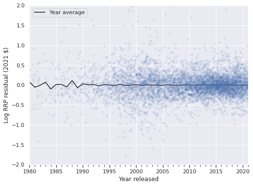

The residuals are reasonably well-centered around zero when grouped by piece and year as expected from the previous post.

Adding subtheme-based random effects and slopes

We now encode subthemes as integer identifiers.

sub_id, sub_map = df["Subtheme"].factorize(sort=True)
n_sub = sub_map.size

sub_id_ = shared(sub_id)

Note that factorize encodes null values as -1 by default, so we see that the number of such entries in sub_id matches the number of sets with null subtheme.

(sub_id == -1).sum()

(df["Subtheme"]
   .isnull()
   .sum())

We build a mask indicating which subthemes are null.

sub_isnull = sub_id == -1
sub_isnull_ = shared(sub_isnull)

We also calculate the average (standardized) log number of pieces for each set in a subtheme.

sub_mean_std_log_pieces = (pd.Series(std_log_pieces, index=df.index)
                             .groupby(df["Subtheme"])
                             .mean())

Recall from the previous post that $j(i)$ represents the index of the theme of the $i$-th set. In similar fashion, let $k(i)$ denote the index of the subtheme of the $i$-th set.

Our model with additional random effects and slopes for subthemes is as follows.

The expected value of the slope is $\beta_0^0 \sim N(0, 2.5^2)$.

with pm.Model() as sub_model:
    β0_0 = pm.Normal("β0_0", 0., 2.5)

The time-varying component of the intercept is

\[\beta_{0, t} \sim \text{GaussianRandomWalk}\left(0, (0.1)^2\right).\]

with sub_model:
    β0_t = gaussian_random_walk("β0_t", n_year, innov_scale=0.1)

\[ \begin{align*} \gamma_0 & \sim N(0, 2.5^2) \\ \sigma_0^{\text{theme}} & \sim \textrm{HalfNormal}(2.5^2) \\ \beta_{0, j}^{\text{theme}} & \sim N\left(\gamma_0 \cdot \bar{\tilde{x}}_j, \left(\sigma_0^{\text{theme}}\right)^2\right). \end{align*} \]

Recall that here $\tilde{x}_i$ is the standardized log piece count of the $i$-th set and $\bar{\tilde{x}}_j$ is the average standardized log piece count of all sets in the $j$-th theme.

with sub_model:
    β0_theme = hierarchical_normal_with_mean(
        "β0_theme",
        at.constant(theme_mean_std_log_pieces),
        n_theme, μ=0.
    )

We now include the sub-theme based random intercepts. All sets with null subtheme are given the same subtheme effect, $\beta_{0, -1}^{\text{sub}}$. We use

\[ \begin{align*} \beta_{0, -1}^{\text{sub}}, \lambda_0^{\text{pieces}} & \sim N(0, 2.5^2) \\ \sigma_0^{\text{sub}} & \sim \text{HalfNormal}(2.5^2) \\ \beta_{0, k}^{\text{sub}} & \sim N\left(\lambda_0^{\text{pieces}} \cdot \check{\tilde{x}}_k, \left(\sigma_0^{\text{sub}}\right)^2\right). \end{align*} \]

Here $\check{\tilde{x}}_k$ is the average standardized log piece count of all sets in the $k$-th subtheme.

with sub_model:
    β0_sub_null = pm.Normal("β0_sub_null", 0., 2.5)
    β0_sub_nn = hierarchical_normal_with_mean(
        "β0_sub_nn",
        at.constant(sub_mean_std_log_pieces),
        n_sub, μ=0., mean_name="λ"
    )
    β0_sub_i = at.switch(
        sub_isnull_,
        β0_sub_null,
        β0_sub_nn[at.clip(sub_id_, 0, n_sub)]
    )

Assembling the intercept terms, we get

\[\beta_{0, i} = \beta_{0, 0} + \beta_{0, t(i)} + \beta_{0, j(i)}^{\text{theme}} + \beta_{0, k(i)}^{\text{sub}}.\]

with sub_model:
    β0_i = β0_0 + β0_t[t_] + β0_theme[theme_id_] + β0_sub_i

The varying slopes, $\beta_{\text{pieces}, i}$, are defined similarly, just without a time-varying component.

with sub_model:
    β_pieces_0 = pm.Normal("β_pieces_0", 0., 2.5)
    
    β_pieces_theme = hierarchical_normal_with_mean(
        "β_pieces_theme",
        at.constant(theme_mean_std_log_pieces),
        n_theme, μ=0.
    )
    
    β_pieces_sub_null = pm.Normal("β_pieces_sub_null", 0., 2.5)
    β_pieces_sub_nn = hierarchical_normal_with_mean(
        "β_pieces_sub_nn",
        at.constant(sub_mean_std_log_pieces),
        n_sub, μ=0., mean_name="λ"
    )
    β_pieces_sub_i = at.switch(
        sub_isnull_,
        β_pieces_sub_null,
        β_pieces_sub_nn[at.clip(sub_id_, 0, n_sub)]
    )

    β_pieces_i = β_pieces_0 + β_pieces_theme[theme_id_] + β_pieces_sub_i

Finally, we specify the likelihood of this model and sample from its posterior distribution.

with sub_model:
    σ = pm.HalfNormal("σ", 5.)
    μ = β0_i + β_pieces_i * std_log_pieces_ - 0.5 * σ**2
    
    obs = pm.Normal("obs", μ, σ, observed=log_rrp2021)

with sub_model:
    sub_trace = pm.sample(**SAMPLE_KWARGS)

Auto-assigning NUTS sampler...
Initializing NUTS using jitter+adapt_diag...
Multiprocess sampling (3 chains in 3 jobs)
NUTS: [β0_0, Δ_β0_t, γ_β0_theme, Δ__β0_theme, σ__β0_theme, β0_sub_null, λ_β0_sub_nn, Δ__β0_sub_nn, σ__β0_sub_nn, β_pieces_0, γ_β_pieces_theme, Δ__β_pieces_theme, σ__β_pieces_theme, β_pieces_sub_null, λ_β_pieces_sub_nn, Δ__β_pieces_sub_nn, σ__β_pieces_sub_nn, σ]

100.00% [6000/6000 17:10<00:00 Sampling 3 chains, 0 divergences]

Sampling 3 chains for 1_000 tune and 1_000 draw iterations (3_000 + 3_000 draws total) took 1031 seconds.
The number of effective samples is smaller than 25% for some parameters.

The sampling diagnostics show no cause for concern.

plot_diagnostics(sub_trace);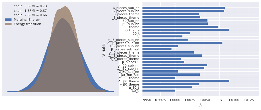

We now sample from the posterior predictive distribution of the model and compare the resulting residuals to those of the baseline model.

with sub_model:
    pp_sub_data = pm.sample_posterior_predictive(sub_trace)

df["sub_pred"] = pp_sub_data["obs"].mean(axis=0)
df["sub_resid"] = log_rrp2021 - df["sub_pred"]

100.00% [3000/3000 00:02<00:00]

fig, (ax, sub_ax) = plt.subplots(
    ncols=2, sharex=True, sharey=True,
    figsize=(2 * FIGSIZE[0], FIGSIZE[1])
)

sns.scatterplot(x="Pieces", y="resid",
                data=df.reset_index(),
                color='C0', alpha=0.1,
                ax=ax);
(df.groupby(df["Pieces"].round(-2))
   ["resid"]
   .mean()
   .plot(c='k', label="Bucketed average",
         ax=ax));

ax.set_xscale('log');

ax.set_ylim(-2, 2);
ax.set_ylabel("Log RRP residual (2021 $)");

ax.legend(loc='upper left');
ax.set_title("Baseline model");

sns.scatterplot(x="Pieces", y="sub_resid",
                data=df.reset_index(),
                color='C0', alpha=0.1,
                ax=sub_ax);
(df.groupby(df["Pieces"].round(-2))
   ["sub_resid"]
   .mean()
   .plot(c='k', ax=sub_ax));

sub_ax.set_title("Subtheme model");

fig.tight_layout();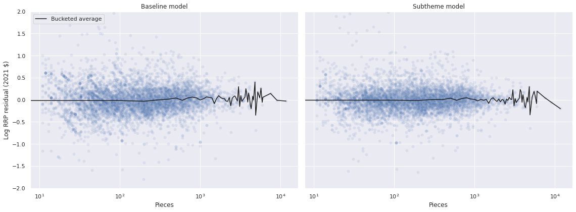

fig, (ax, sub_ax) = plt.subplots(
    ncols=2, sharex=True, sharey=True,
    figsize=(2 * FIGSIZE[0], FIGSIZE[1])
)

(df.groupby(level="Year released")
   ["resid"]
   .mean()
   .plot(c='k', label="Year average",
         ax=ax));

strip_ax = ax.twiny()
sns.stripplot(x="Year released", y="resid",
              data=df.reset_index(),
              jitter=1.5,
              color='C0', alpha=0.1,
              ax=strip_ax);

strip_ax.set_axis_off();

ax.set_ylim(-2, 2);
ax.set_ylabel("Log RRP residual (2021 $)");

ax.legend(loc='upper left');
ax.set_title("Baseline model");

(df.groupby(level="Year released")
   ["sub_resid"]
   .mean()
   .plot(c='k', label="Year average",
         ax=sub_ax));

sub_strip_ax = sub_ax.twiny()
sns.stripplot(x="Year released", y="sub_resid",
              data=df.reset_index(),
              jitter=1.5,
              color='C0', alpha=0.1,
              ax=sub_strip_ax);

sub_strip_ax.set_axis_off();

sub_ax.set_title("Subtheme model");

fig.tight_layout();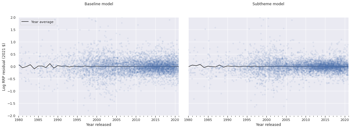

The residuals look quite similar, with perhaps slightly less variation for the subtheme model. Since the residuals are so visually similar, we turn to Pareto-smoothed importance sampling leave-one-out cross validation¹ (PSIS-LOO) to compare the models.

traces = {
    "Baseline": trace,
    "Subtheme": sub_trace
}

%%time
comp_df = az.compare(traces)

CPU times: user 20.7 s, sys: 397 ms, total: 21.1 s
Wall time: 21.1 s

comp_df.loc[:, :"weight"]

	rank	loo	p_loo	d_loo	weight
Subtheme	0	-1142.927746	639.913733	0.000000	0.911548
Baseline	1	-2062.767732	251.538394	919.839986	0.088452

az.plot_compare(comp_df, plot_ic_diff=False);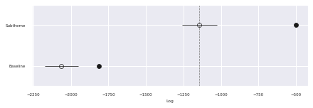

We see that the subtheme model has approximately 2.5 times as many effective parameters as the baseline model and produces a significantly higher PSIS-LOO score.

Model interpretation

We now interpret the posterior distributions of various parameters and the posterior predictions of these two models.

LARGE_LABEL_FS = 18

grid = az.plot_posterior(
    trace,
    var_names=[
        "σ__β0_theme",
        "σ__β_pieces_theme"
    ],
    hdi_prob='hide',
    color='C0', label="Baseline model"
)
az.plot_posterior(
    sub_trace,
    var_names=[
        "σ__β0_theme",
        "σ__β_pieces_theme"
    ],
    hdi_prob='hide',
    color='C1', label="Subtheme model",
    ax=grid
);

grid[0].set_xlabel(r"$\sigma_{\beta_0^{\mathrm{theme}}}$",
                   fontsize=LARGE_LABEL_FS);
grid[0].set_title(None);
grid[0].get_legend().remove()

grid[1].set_xlabel(r"$\sigma_{\beta_{\mathrm{pieces}}^{\mathrm{theme}}}$",
                   fontsize=LARGE_LABEL_FS);
grid[1].set_title(None);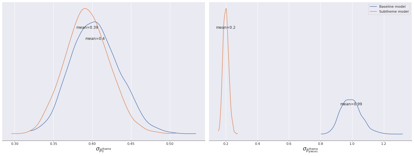

We see that after adding subtheme-based varying intercepts and slopes that the scale of the varying intercepts remains roughly the same, but the scale of the varying slopes is greatly reduced.

grid = az.plot_posterior(sub_trace,
                         var_names=[
                            "σ__β0_sub_nn",
                            "σ__β_pieces_sub_nn"
                         ])

grid[0].set_xlabel(r"$\sigma_{\beta_0^{\mathrm{sub}}}$",
                   fontsize=18);
grid[0].set_title(None);

grid[1].set_xlabel(r"$\sigma_{\beta_{\mathrm{pieces}}^{\mathrm{sub}}}$",
                   fontsize=18);
grid[1].set_title(None);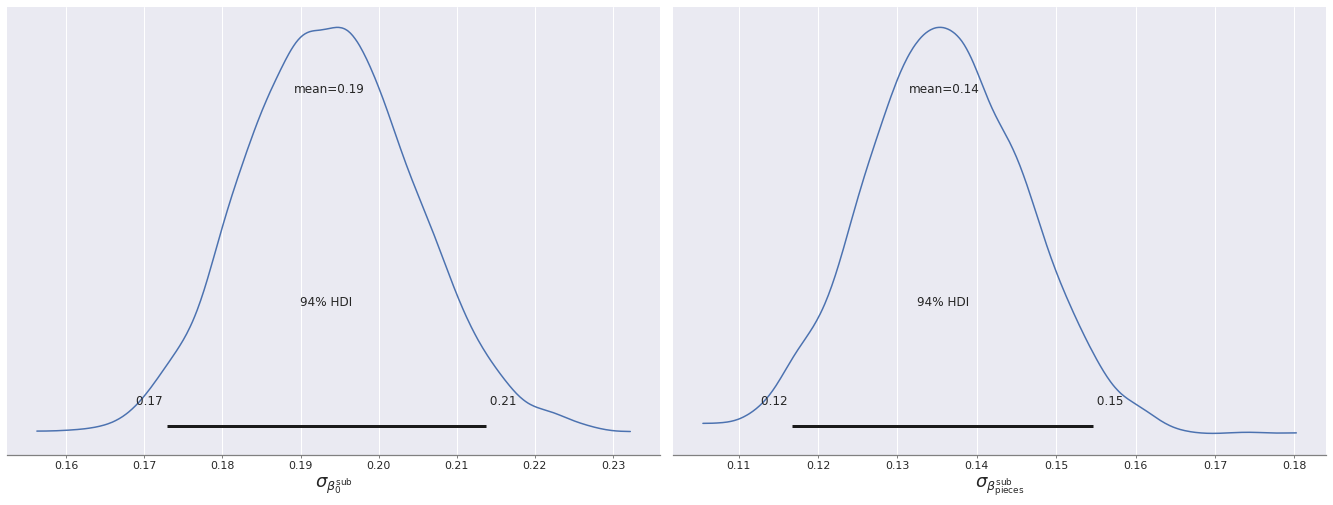

Interestingly, the scale of the subtheme-based variation is significantly smaller than that of the theme-based variation in the baseline model.

β0_theme_hat = trace["posterior"]["β0_theme"].mean(dim=("chain", "draw"))
β_pieces_theme_hat = trace["posterior"]["β_pieces_theme"].mean(dim=("chain", "draw"))

β0_theme_hat_sub = sub_trace["posterior"]["β0_theme"].mean(dim=("chain", "draw"))
β_pieces_theme_hat_sub = sub_trace["posterior"]["β_pieces_theme"].mean(dim=("chain", "draw"))

fig, (int_ax, slope_ax) = plt.subplots(
    ncols=2,
    figsize=(2 * FIGSIZE[1], FIGSIZE[1])
)

int_ax.set_aspect('equal');
slope_ax.set_aspect('equal');

sns.scatterplot(
    x=β0_theme_hat, y=β0_theme_hat_sub,
    alpha=0.5, ax=int_ax
);

int_ax.axline((0, 0), slope=1, c='k', ls='--');

int_ax.set_xlabel("Baseline model");
int_ax.set_ylabel("Subtheme model");
int_ax.set_title(r"$\beta_0^{\mathrm{theme}}$");

sns.scatterplot(
    x=β_pieces_theme_hat, y=β_pieces_theme_hat_sub,
    alpha=0.5, ax=slope_ax
);

slope_ax.axline((0, 0), slope=1, c='k', ls='--');

slope_ax.set_xlabel("Baseline model");
slope_ax.set_ylabel("Subtheme model");
slope_ax.set_title(r"$\beta_{\mathrm{pieces}}^{\mathrm{theme}}$");

fig.tight_layout();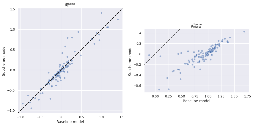

These relationships are shown clearly when we scatter plot the posterior expected value of the theme-based varying slopes and intercepts against each other from each model. We see that the theme-based varying intercepts are largely concentrated around the line $y = x$ while the theme-based varying slopes almost all have $y < x$.

β0_sub_nn_hat = sub_trace["posterior"]["β0_sub_nn"].mean(dim=("chain", "draw"))
β_pieces_sub_nn_hat = sub_trace["posterior"]["β_pieces_sub_nn"].mean(dim=("chain", "draw"))

ax = sns.scatterplot(
    x=β0_sub_nn_hat, y=β_pieces_sub_nn_hat,
    alpha=0.5
)

ax.set_xlabel(r"$\beta_0^{\mathrm{sub}}$");
ax.set_ylabel(r"$\beta_{\mathrm{pieces}}^{\mathrm{sub}}$");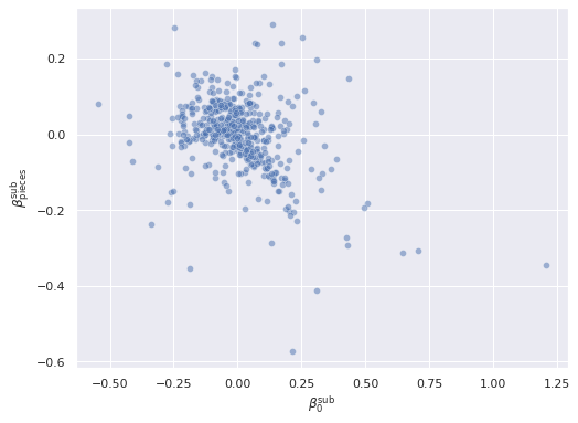

There is a negative relationship subtheme-based varying intercepts and slopes. As the subtheme-based intercept increased, the subtheme-based slope decreases.

fig, (int_ax, slope_ax) = plt.subplots(
    ncols=2,
    figsize=(2 * FIGSIZE[1], FIGSIZE[1])
)

sns.scatterplot(
    x=β0_theme_hat, y=β_pieces_theme_hat,
    alpha=0.5, ax=int_ax
);

int_ax.set_xlabel(r"$\beta_0^{\mathrm{theme}}$");
int_ax.set_ylabel(r"$\beta_{\mathrm{pieces}}^{\mathrm{theme}}$");
int_ax.set_title("Baseline model");

sns.scatterplot(
    x=β0_theme_hat_sub, y=β_pieces_theme_hat_sub,
    alpha=0.5, ax=slope_ax
);

slope_ax.set_xlabel(r"$\beta_0^{\mathrm{theme}}$");
slope_ax.set_ylabel(r"$\beta_{\mathrm{pieces}}^{\mathrm{theme}}$");
slope_ax.set_title("Subtheme model");

fig.tight_layout();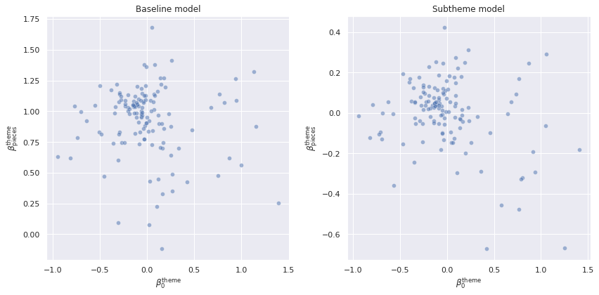

These negative relationships exist for the theme-based varying intercepts and slopes in both models as well, but are less pronounced. This tighter relationship between subtheme-based varying intercepts and slopes is partially responsible for the smaller scale of the theme-based varying slopes in the subtheme model.

We now turn to examining the effects of particular subthemes. First we plot the subthemes with the most extreme intercept and slopes.

N_EXTREME = 10

def get_extreme_ix(x, n_extreme=N_EXTREME):
    argsorted = x.argsort()
    
    return np.concatenate((argsorted[:n_extreme // 2], argsorted[-(n_extreme // 2):]))

β0_sub_ext_ix = get_extreme_ix(β0_sub_nn_hat)

ax, = az.plot_forest(sub_trace, var_names=["β0_sub_nn"],
                     coords={
                       "β0_sub_nn_dim_0": β0_sub_ext_ix
                     },
                     hdi_prob=0.95, combined=True)

ax.set_xlabel(r"$\beta_0^{\mathrm{sub}}$");
ax.set_yticklabels(sub_map[β0_sub_ext_ix][::-1]);
ax.set_title(None);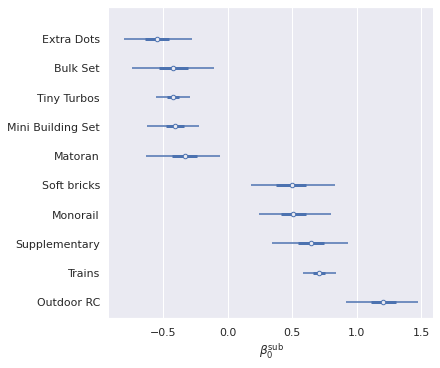

β_pieces_sub_ext_ix = get_extreme_ix(β_pieces_sub_nn_hat)

ax, = az.plot_forest(sub_trace, var_names=["β_pieces_sub_nn"],
                     coords={
                       "β_pieces_sub_nn_dim_0": β_pieces_sub_ext_ix
                     },
                     hdi_prob=0.95, combined=True)

ax.set_xlabel(r"$\beta_{\mathrm{pieces}}^{\mathrm{sub}}$");
ax.set_yticklabels(sub_map[β_pieces_sub_ext_ix][::-1]);
ax.set_title(None);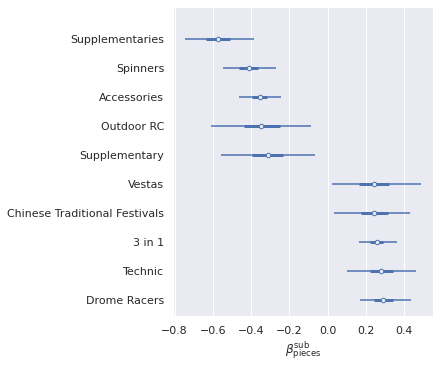

That subthemes like “Extra Dots,” “Bulk Set,” and “Mini Building Set” have some of the smallest intercepts and “Outdoor RC” has the largest is intuitive. Due to the negative correlation between subtheme intercepts and slopes, we then see that “Outdoor RC” is in the bottom in terms of slope. It also makes sense that “Technic” has one of the highest slopes, as Technic sets tend to include specialized pieces more often than most subthemes.

The Republic Gunship

We now return to the original question in this post, whether the Ultimate Collector Series Republic Gunship is fairly priced. To answer this question, first we examine the varying slopes and intercepts for Star Wars-themed and Ultimate Collector Series-subthemed sets for the models.

star_wars_id = (theme_map == STAR_WARS).argmax()

grid = az.plot_posterior(
    trace,
    var_names=[
        "β0_theme",
        "β_pieces_theme"
    ],
    coords={
        "β0_theme_dim_0": [star_wars_id],
        "β_pieces_theme_dim_0": [star_wars_id]
    },
    hdi_prob='hide',
    color='C0', label="Baseline model"
)
az.plot_posterior(
    sub_trace,
    var_names=[
        "β0_theme",
        "β_pieces_theme"
    ],
    coords={
        "β0_theme_dim_0": [star_wars_id],
        "β_pieces_theme_dim_0": [star_wars_id]
    },
    hdi_prob='hide',
    color='C1', label="Subtheme model",
    ax=grid
);

grid[0].set_xlabel(r"$\beta_0^{\mathrm{theme}}$",
                   fontsize=LARGE_LABEL_FS);
grid[0].set_title(None);
grid[0].get_legend().remove()

grid[1].set_xlabel(r"$\beta_{\mathrm{pieces}}^{\mathrm{theme}}$",
                   fontsize=LARGE_LABEL_FS);
grid[1].set_title(None);

plt.gcf().suptitle("Star Wars");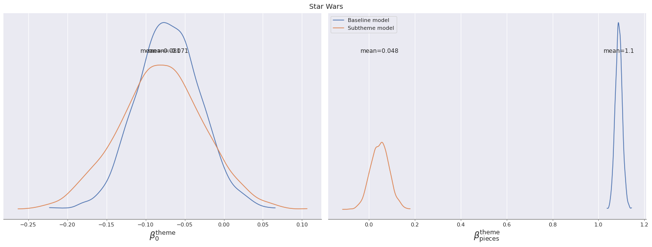

As with the general trend, we see that the posterior distributions for the intercept Star Wars-themed sets are similar for both models, but their slopes are quite different.

UCS = "Ultimate Collector Series"
ucs_id = (sub_map == UCS).argmax()

We see that the intercept for Ultimate Collector series sets is quite average and the slope for such sets is perhaps slightly positive, but not large.

int_ax, slope_ax = az.plot_posterior(
    sub_trace,
    var_names=[
        "β0_sub_nn",
        "β_pieces_sub_nn"
    ],
    coords={
        "β0_sub_nn_dim_0": [ucs_id],
        "β_pieces_sub_nn_dim_0": [ucs_id]
    },
    ref_val=0.
)

int_ax.set_xlabel(r"$\beta_0^{\mathrm{sub}}$",
                  fontsize=LARGE_LABEL_FS);
int_ax.set_title(None);

slope_ax.set_xlabel(r"$\beta_{\mathrm{pieces}}^{\mathrm{sub}}$",
                    fontsize=LARGE_LABEL_FS);
slope_ax.set_title(None);

plt.gcf().suptitle("Ultimate Collector Series");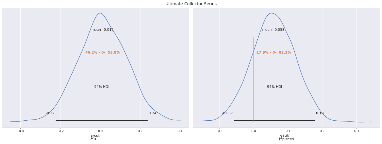

We see that Ultimate Collector series sets are not really set apart by their subtheme intercept or slope, but rather the fact that they have many more pieces than most Star WSars sets (on average).

ax = sns.kdeplot(df["Pieces"][df["Theme"] == STAR_WARS],
                 clip=(0., np.inf),
                 label="All Star Wars sets")
sns.kdeplot(df["Pieces"][df["Subtheme"] == UCS],
            clip=(0., np.inf),
            label="Ultimate Collector Series sets",
            ax=ax);
sns.rugplot(df["Pieces"][df["Subtheme"] == UCS],
            height=0.05, c='C1', ax=ax);

ax.set_xlim(left=-100.);
ax.set_yticklabels([]);
ax.legend();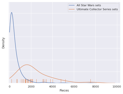

Finally we examine the posterior predictive distribution of the price of the Ultimate Collector Series Republic Gunship.

GUNSHIP_SET_NUM = "73509"
GUNSHIP_PIECES = 3292

GUNSHIP_YEAR = 2021
gunship_t = 2021 - year.min()

std_log_pieces_.set_value(scale_log_pieces(np.log([GUNSHIP_PIECES])))
theme_id_.set_value([star_wars_id])
sub_isnull_.set_value([False])
sub_id_.set_value([ucs_id])
t_.set_value([gunship_t])

with model:
    pp_gunship_data = pm.sample_posterior_predictive(trace)

100.00% [3000/3000 00:00<00:00]

with sub_model:
    pp_gunship_sub_data = pm.sample_posterior_predictive(sub_trace)

100.00% [3000/3000 00:00<00:00]

GUNSHIP_RRP = 349.99

def format_posterior_artist(artist, formatter):
    text = artist.get_text()
    x, _ = artist.get_position()

    if text.startswith(" ") or text.endswith(" "):
        fmtd_text = formatter(x)
        artist.set_text(
            " " + fmtd_text if text.startswith(" ") else fmtd_text + " "
        )
    elif "=" in text:
        before, _ = text.split("=")
        artist.set_text("=".join((before, formatter(x))))
    elif "<" in text:
        below, ref_val_str, above = text.split("<")
        artist.set_text("<".join((
            below,
            " " + formatter(float(ref_val_str)) + " ",
            above
        )))

def format_posterior_text(formatter, ax=None):
    if ax is None:
        ax = plt.gca()
    
    artists = [artist for artist in ax.get_children() if isinstance(artist, plt.Text)]
    
    for artist in artists:
        format_posterior_artist(artist, formatter),

fig, (ax, sub_ax) = plt.subplots(
    ncols=2, sharex=True, sharey=True,
    figsize=(2 * FIGSIZE[0], FIGSIZE[1]))

az.plot_posterior(np.exp(pp_gunship_data["obs"]),
                  ref_val=GUNSHIP_RRP, ax=ax);
format_posterior_text(dollar_formatter, ax=ax)

ax.set_xlabel(f"Posterior predicted RRP for {GUNSHIP_SET_NUM}\n(2021 $)");
ax.set_title("Baseline model");

az.plot_posterior(np.exp(pp_gunship_sub_data["obs"]),
                  ref_val=GUNSHIP_RRP, ax=sub_ax);
format_posterior_text(dollar_formatter, ax=sub_ax)

sub_ax.set_xlabel(f"Posterior predicted RRP for {GUNSHIP_SET_NUM}\n(2021 $)");
sub_ax.set_title("Subtheme model");

fig.tight_layout();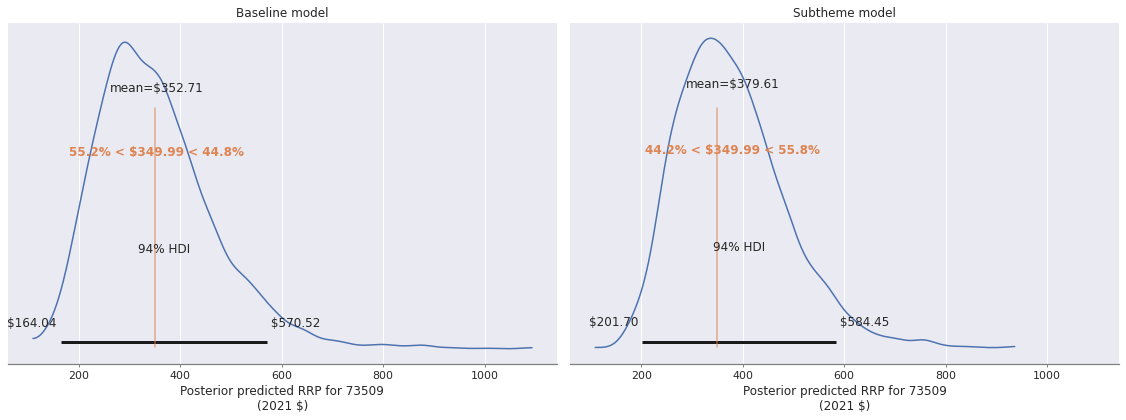

The plot on the left shows that the baseline model considers the Ultimate Collector Series Republic Gunship slightly overpriced, while the plot on the right shows that the subtheme model considers it slightly underpriced. Since these deviations from the posterior expected value are small in either case, it is safe to say that both of these models consider the Ultimate Collector Series Republic Gunship to be priced in line with Lego’s historic prices. (I’ll be ordering it come August 1.)

This post is available as a Jupyter notebook here.

%load_ext watermark
%watermark -n -u -v -iv

Last updated: Tue Jul 20 2021

Python implementation: CPython
Python version       : 3.7.10
IPython version      : 7.24.1

aesara    : 2.0.12
seaborn   : 0.11.1
numpy     : 1.19.5
pymc3     : 4.0
matplotlib: 3.4.2
arviz     : 0.11.2
pandas    : 1.2.4

Vehtari, A., Gelman, A., & Gabry, J. (2017). Practical Bayesian model evaluation using leave-one-out cross-validation and WAIC. Statistics and computing, 27(5), 1413-1432.↩︎