Prior Distributions for Bayesian Regression Using PyMC

In this post, I’ll discuss the basics of Bayesian linear regression, exploring three different prior distributions on the regression coefficients. The models in question are defined by the equation

$$y = x^T \beta + \varepsilon$$

for $x, \beta \in \mathbb{R}^p$ and $\varepsilon \sim N(0, \sigma^2),$ where $\sigma^2$ is known. In this example, we will use $\sigma^2 = 1.$ If we have observed $x_1, \ldots, x_n \in \mathbb{R}^p$, the conditional distribution is $y | X, \beta \sim N(X \beta, \sigma^2 I),$ where

$$X = \begin{pmatrix} x_1^T \\ \vdots \\ x_n^T \end{pmatrix} \in \mathbb{R}^{n \times p}$$

and

$$y = \begin{pmatrix} y_1 \\ \vdots \\ y_n \end{pmatrix} \in \mathbb{R}^n.$$

To determine the regression coefficients, we will use maximum a posteriori esimation (MAP), which is the Bayesian counterpart of maximum likelihod estimation. The MAP estimate of a quantity is the value with the largest posterior likelihood. Before we can estimate the regression coefficients in this manner, we must place a prior distribution on them. We will explore three different choices of prior distribution and the Bayesian approaches to which they each lead.

We will use each approach to examine data generated according to a model from the excellent blog post Machine Learning Counterexamples Part 1 by Cam Davison-Pilon. The data are generated according to the relation

$$y = 10 x_1 + 10 x_2 + 0.1 x_3,$$

where $x_1 \sim N(0, 1)$, $x_2 = -x_1 + N(0, 10^{-6})$, and $x_3 \sim N(0, 1)$. We now generate data according to this model.

from scipy.stats import norm

n = 1000

x1 = norm.rvs(0, 1, size=n)
x2 = -x1 + norm.rvs(0, 10**-3, size=n)
x3 = norm.rvs(0, 1, size=n)

X = np.column_stack([x1, x2, x3])
y = 10 * x1 + 10 * x2 + 0.1 * x3

Since $x_1$ and $x_2$ are highly correlated, we see that the model reduces to

$$y = 0.1 x_3 + N(0, 10^{-6}).$$

Each of the priors on the regression coefficients will predict this reduced model with varying amounts of accuracy. When estimating the regression coefficients, we assume the model has the form

$$y = \beta_1 x_1 + \beta_2 x_2 + \beta_3 x_3,$$

so the correct values of the coefficients are $\beta_1 = 0 = \beta_2$ and $\beta_3 = 0.1.$

Ordinary Least Squares

The simplest choice is the improper, un informative prior $\pi(\beta) = 1$ for $\beta \in \mathbb{R}^p.$

import matplotlib.pyplot as plt

xmax = 1000

fig = plt.figure()
ax = fig.add_subplot(111)
ax.plot((-xmax, xmax), (1, 1));
ax.set_ylim(bottom=0);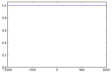

This prior reflects a belief that all possible values of the regression coefficients are equally likely. It also induces significant simplication in Bayes’ Theorem:

$$\begin{array} {}f(\beta | y, X) & = \frac{f(y | X, \beta) \pi(\beta)}{\int_{-\infty}^\infty f(y | X, \beta) \pi(\beta)\ d \beta} \\ & = \frac{f(y | X, \beta)}{\int_{-\infty}^\infty f(y | X, \beta) \ d \beta}. \end{array}$$

The MAP estimate of $\beta$ is

$$\begin{array} {}\hat{\beta}_{MAP} & = \operatorname{max}_\beta f(\beta | y, X) \\ & = \operatorname{max}_\beta \frac{f(y | X, \beta)}{\int_{-\infty}^\infty f(y | X, \beta) \ d \beta} \\ & = \operatorname{max}_\beta f(y | X, \beta), \end{array}$$

since the value of the integral is positive and does not depend on $\beta$. We see that with the uninformative prior $\pi(\beta) = 1$, the MAP estimate coincides with the maximum likelihood estimate.

It is well-known that the maximum likelihood estimate of $\beta$ is the ordinary least squares estimate, $\hat{\beta}_{OLS} = (X^T X)^{-1} X^T y.$

import numpy as np

np.dot(np.dot(np.linalg.inv(np.dot(X.T, X)), X.T), y)

array([ 10. ,  10. ,   0.1])

We see here that ordinary least squares regression recovers the full model, $y = 10 x_1 + 10 x_2 + 0.1 x_3$, not the more useful reduced model. The reason that ordinary least squares results in the full model is that it assumes the regressors are independent, and therefore cannot account for the fact that $x_1$ and $x_2$ are highly correlated.

In order to derive the least squares coefficients from the Bayesian perspective, we must define the uninformative prior in pymc.

import pymc
import sys

beta_min = -10**6
beta_max = 10**6

beta1_ols = pymc.Uniform(name='beta1', lower=beta_min, upper=beta_max)
beta2_ols = pymc.Uniform(name='beta2', lower=beta_min, upper=beta_max)
beta3_ols = pymc.Uniform(name='beta3', lower=beta_min, upper=beta_max)

Here we use uniform distributions with support of $[-10^6, 10^6]$ to approximate the uninformative prior while avoiding arithmetic overflows.

Now we define the linear predictor in terms of the coefficients $\beta_1$, $\beta_2$, and $\beta_3$.

@pymc.deterministic
def y_hat_ols(beta1=beta1_ols, beta2=beta2_ols, beta3=beta3_ols, x1=x1, x2=x2, x3=x3):
    return beta1 * x1 + beta2 * x2 + beta3 * x3

Note that we have applied the pymc.deterministic decorator to y_hat_ols because it is a deterministic function of its inputs, even though these inputs are stochastic. We now define the response variable, pass its values to pymc, and indicate that these values were observed and therefore are fixed.

Y_ols = pymc.Normal(name='Y', mu=y_hat_ols, tau=1.0, value=y, observed=True)

We now initialze the pymc model and maximup a posteriori fitter.

ols_model = pymc.Model([Y_ols, beta1_ols, beta2_ols, beta3_ols])
ols_map = pymc.MAP(ols_model)
ols_map.fit()

We now retrieve the maximum a posteriori values of the coefficients.

def get_coefficients(map_):
    return [{str(variable): variable.value} for variable in map_.variables if str(variable).startswith('beta')]

get_coefficients(ols_map)

[{'beta2': array(10.00004405085075)},
 {'beta1': array(10.000044044812622)},
 {'beta3': array(0.10000003820538296)}]

We see that these values are within the algorithm’s step sizes,

ols_map.eps

array([ 0.001,  0.001,  0.001])

of the explicitly calculated ordinary least squares regression coefficients.

Ridge Regression

The uninformative prior represents the belief that all combinations of regression coefficients are equally likely. In practice, this assumption is often not justified, and we may have reason to believe that many (or even most) of the regressors have little to no impact on the response. Such a belief can be interpreted as a preference for simple models with fewer regressors.

Given that the normal distribution is among the most studied objects in mathematics, a reasonable approach to quantifying this belief is to place zero-mean normal priors on the regression coefficients to indicate our preference for smaller values. This choice of prior distribution gives rise to the technique of ridge regression.

xs = np.linspace(-5, 5, 250)

fig = plt.figure()
ax = fig.add_subplot(111)
ax.plot(xs, norm.pdf(xs));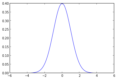

We now use pymc to give the coefficients standard normal priors.

beta1_ridge = pymc.Normal('beta1', mu=0, tau=1.0)
beta2_ridge = pymc.Normal('beta2', mu=0, tau=1.0)
beta3_ridge = pymc.Normal('beta3', mu=0, tau=1.0)

Just as with ordinary least squares, we define our linear predictor in terms of these coefficients.

@pymc.deterministic
def y_hat_ridge(beta1=beta1_ridge, beta2=beta2_ridge, beta3=beta3_ridge, x1=x1, x2=x2, x3=x3):
    return beta1 * x1 + beta2 * x2 + beta3 * x3

We also set the distribution of the response.

Y_ridge = pymc.Normal('Y', mu=y_hat_ridge, tau=1.0, value=y, observed=True)

Again, we fit the model and find the MAP estimates.

ridge_model = pymc.Model([Y_ridge, beta1_ridge, beta2_ridge, beta3_ridge])
ridge_map = pymc.MAP(ridge_model)
ridge_map.fit()

get_coefficients(ridge_map)

[{'beta1': array(0.004539760042452516)},
 {'beta2': array(0.004743440885490875)},
 {'beta3': array(0.09987676239942628)}]

These estimates are much closer the the reduced model, $y = 0.1 x_3 + \varepsilon$, than the ordinary least squares estimates. The coefficients $\beta_1$ and $\beta_2$, however, differ from their true values of zero by more than the aglorithm’s step sizes,

ridge_map.eps

array([ 0.001,  0.001,  0.001])

To be thorough, let’s compare these estimates to those computed by scikit- learn.

from sklearn.linear_model import RidgeCV

skl_ridge_model = RidgeCV(fit_intercept=False)
skl_ridge_model.fit(X, y)
skl_ridge_model.coef_

array([ 0.04630535,  0.04650529,  0.0999703 ])

These values are quite close to those produced by pymc.

The reason that the ridge estimates of the regression coefficients are close to the true model, but not quite exactly in line with it, is that the standard normal prior causes all of the regression coefficients to shrink towards zero. While it is correct to shrink $\beta_1$ and $\beta_2$ to zero, this shrinkage must be balanced with the fact that $\beta_3$ is nonzero.

LASSO Regression

The final Bayesian regression method we consider in this post is the LASSO. It is also based off the prior belief that most coefficients should be (close to) zero, but expresses this belief through a different, more exotic, prior distribution.

The prior in question is the Laplace distribution (also known as the double exponential distribution). The following diagram contrasts the probability density functions of the normal distribution and the Laplace distribution.

from scipy.stats import laplace

sigma2 = 1.0
b = 1.0 / np.sqrt(2.0 * sigma2)

fig = plt.figure()
ax = fig.add_subplot(111)
ax.plot(xs, norm.pdf(xs), label='Normal');
ax.plot(xs, laplace.pdf(xs, shape=b), label='Laplace');
ax.legend();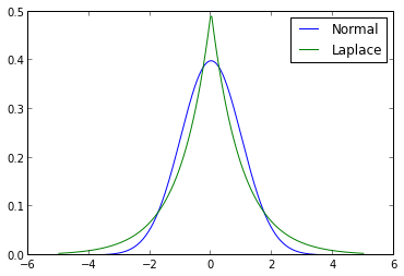

The shape parameter of the Laplace distribution in this figure was chosen so that it would have unit variance, the same as the normal distribution shown.

The first notable feature of this diagram is that the Laplace distribution assigns a higher density to a neighborhood of zero than the normal distribution does. This fact serves to strengthen our prior assumption that the regression coefficients are likely to be zero. The second notable feature is that the Laplace distribution has fatter tails than the normal distribution, which will cause it to shrink all coefficients less than the normal prior does in ridge regression.

We now fit the LASSO model in pymc.

beta1_lasso = pymc.Laplace('beta1', mu=0, tau=1.0 / b)
beta2_lasso = pymc.Laplace('beta2', mu=0, tau=1.0 / b)
beta3_lasso = pymc.Laplace('beta3', mu=0, tau=1.0 / b)

@pymc.deterministic
def y_hat_lasso(beta1=beta1_lasso, beta2=beta2_lasso, beta3=beta3_lasso, x1=x1, x2=x2, x3=x3):
    return beta1 * x1 + beta2 * x2 + beta3 * x3

Y_lasso = pymc.Normal('Y', mu=y_hat_lasso, tau=1.0, value=y, observed=True)

lasso_model = pymc.Model([Y_lasso, beta1_lasso, beta2_lasso, beta3_lasso])
lasso_map = pymc.MAP(lasso_model)
lasso_map.fit()

get_coefficients(lasso_map)

[{'beta2': array(-9.289356796847342e-06)},
 {'beta3': array(0.09870141129637913)},
 {'beta1': array(1.811243155314106e-05)}]

These estimates are all within the algorithm’s step size,

map_fitter.eps

array([ 0.001,  0.001,  0.001])

of the reduced model’s true coefficients.

We will once again verify these estimates using scikit-learn.

from sklearn.linear_model import LassoCV

skl_lasso_model = LassoCV(fit_intercept=False)
skl_lasso_model.fit(X, y)
skl_lasso_model.coef_

array([-0.        ,  0.        ,  0.09952034])

These estimates are all fairly close to those produced by pymc. Here we also see one of the differences between the LASSO and ridge regression. While ridge regressionn tends to shrink all coefficients towards zero, the LASSO tends to set some coefficients exactly equal to zero. This behavior is one of the main practical differences between the two regression methods.

Further Exploration

We have only scratched the surface of Bayesian regression and pymc in this post. In my mind, finding maximum a posteriori estimates is only a secondary function of pymc. Its primary function is sampling from posterior distributions using Markov chain Monte Carlo sampling for models whose posteriors are difficult or impossible to calculate explicity.

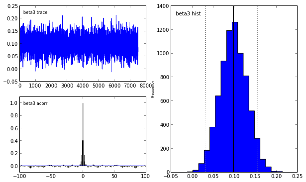
Indeed, our reliance on MAP point estimates obscures one of the most powerful features of Bayesian inference, which is the ability to consider the posterior distribution as a whole. In the case of the LASSO, we may obtain samples from the posterior using pymc in the following manner.

lasso_mcmc = pymc.MCMC(lasso_model)
lasso_mcmc.sample(20000, 5000, 2)

pymc.Matplot.plot(lasso_mcmc)

[****************100%******************]  20000 of 20000 complete
Plotting beta3
Plotting beta2
Plotting beta1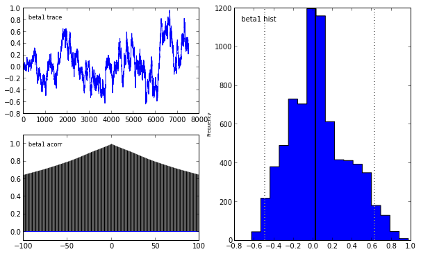

To learn more abouy Bayesian statistis and pymc, I strongly recommend the fantastic open source book Probabilistic Programming and Bayesian Methods for Hackers.

This post is written as an IPython notebook. The notebook is available under the MIT License.