Robust Regression with t-Distributed Residuals
Ordinarly least squares (OLS) is, without a doubt, the most-well known linear regression model. Despite its wide applicability, it often gives undesireable results when the data deviate from its underlying normal model. In particular, it is quite sensitive to outliers in the data. In this post, we will illustrate this sensitivity and then show that changing the error distribution results in a more robust regression model.
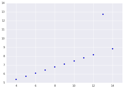
We will use one of the data sets from Anscombe’s quartet to illustrate these concepts. Anscombe’s quartet is a well-known group of four data sets that illustrates the importance of exploratory data analysis and visualization. In particular, we will use the third dataset from Anscombe’s quartet. This data set is shown below.
from matplotlib import pyplot as plt
import numpy as np
import pandas as pd
import pymc3
from scipy import stats
import seaborn as sns
from statsmodels import api as sm
x = np.array([10, 8, 13, 9, 11, 14, 6, 4, 12, 7, 5])
y = np.array([7.46, 6.77, 12.74, 7.11, 7.81, 8.84, 6.08, 5.39, 8.15, 6.42, 5.73])
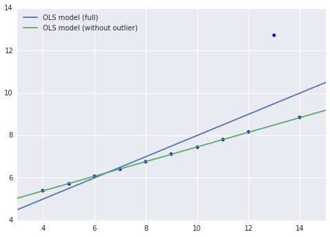
It is quite clear that this data set exhibits a highly linear relationship, with one outlier (when x = 13). Below, we show the results of two OLS models fit to this data. One is fit to all of the data, and the other is fit to the data with the outlier point removed.
X = sm.add_constant(x)ols_result = sm.OLS(y, X).fit()x_no_outlier = x[x != 13]
X_no_outlier = X[x != 13]
y_no_outlier = y[x != 13]no_outlier_result = sm.OLS(y_no_outlier, X_no_outlier).fit()
One of the ways the OLS estimator can be derived is by minimizing the mean squared error (MSE) of the model on the training data. Below we show the MSE of both of these models on both the full data set and the data set without the outlier.
def mse(actual, predicted):
    return ((actual - predicted)**2).mean()
mse_df = pd.DataFrame({
'Full data set': [
mse(y, ols_result.predict(X)),
mse(y, no_outlier_result.predict(X))
],
'Data set without outlier': [
mse(y_no_outlier, ols_result.predict(X_no_outlier)),
mse(y_no_outlier, no_outlier_result.predict(X_no_outlier))
]
},
index=['Full model', 'No outlier mdoel']
)
mse_df = mse_df[mse_df.columns[::-1]]mse_df| Full data set | Data set without outlier | |
|---|---|---|
| Full model | 1.250563 | 0.325152 |
| No outlier mdoel | 1.637640 | 0.000008 |
By simple visual inspection, we suspect that without the outlier (x = 13), the relationship between x and y is (almost) perfectly linear. This suspicion is confirmed by this model’s very small MSE on the reduced data set.
Toward robust regression
Unfortunately, we will usually have many more than eleven points in our data set. In reality, the outliers may be more difficult to detect visually, and they may be harder to exclude manually. We would like a model that performs reasonably well, even in the presence of outliers.
Before we define such a robust regression model, it will be helpful to consider the OLS model mathematically. In the OLS model, we have that
\[y_i = \vec{\beta} \cdot \vec{x}_i + \varepsilon_i.\]
Here, \(y_i\) is the observation corresponding to the feature vector \(\vec{x}_i\), \(\vec{\beta}\) is the vector of regression coefficients, and \(\varepsilon_i\) is noise. In the OLS model, the noise terms are independent with identical normal distributions. It is the properties of these normally distributed errors that make OLS susceptible to outliers.
The normal distribution is well-known to have thin tails. That is, it assigns relatively little probability to observations far away from the mean. Students of basic statistics are quite familiar with the fact that approximately 95% of the mass of the normal distribution lies within two standard deviations of the mean.
We find a robust regression model by choosing an error distribution with fatter tails; a common choice is Student’s t-distribution.
Below we define this model using pymc3.
with pymc3.Model() as model:
    # Regression coefficients
    alpha = pymc3.Uniform('alpha', -100, 100)
    beta = pymc3.Uniform('beta', -100, 100)

    # Expected value
    y_hat = alpha + beta * x

    # Observations with t-distributed error
    y_obs = pymc3.T('y_obs', nu=5, mu=y_hat, observed=y)
Here we have given our t-distributed residuals five degrees of freedom. Customarily, these models will use four, five, or six degrees of freedom. It is important that the number of degrees of freedom, \(\nu\), be relatively small, because as \(\nu \to \infty\), the t-distribution converges to the normal distribution.
We now fit this model using no-U-turn sampling.
with model:
    step = pymc3.NUTS()
    trace_ = pymc3.sample(3000, step)

burn = 1000
thin = 2
trace = trace_[burn::thin]
[-----------------100%-----------------] 3000 of 3000 complete in 8.7 secThe following plots summarize the posterior distribution of the regression intercept (\(\alpha\)) and slope (\(\beta\)).

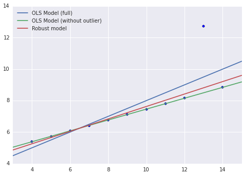
We now plot the robust model along with the previous models.
alpha = trace['alpha'].mean()
beta = trace['beta'].mean()
We see right away that, although the robust model has not completely captured the linear relationship between the non-outlier points, it is much less biased by the outlier than the OLS model on the full data set. Below we compare the MSE of this model to the previous models.
robust_mse = pd.Series([mse(y, alpha + beta * x), mse(y_no_outlier, alpha + beta * x_no_outlier)], index=mse_df.columns)
robust_mse.name = 'Robust model'
mse_df = mse_df.append(robust_mse)mse_df| Full data set | Data set without outlier | |
|---|---|---|
| Full model | 1.250563 | 0.325152 |
| No outlier mdoel | 1.637640 | 0.000008 |
| Robust model | 1.432198 | 0.032294 |
On the data set without the outlier, the robust model has a significantly larger MSE than the no outlier model, but, importantly, its MSE is an order of magnitude smaller than that of the full model.