Saving Memory by Counting Combinations of Features
For all the hype about big data, much value resides in the world’s medium and small data. Especially when we consider the length of the feedback loop and total analyst time invested, insights from small and medium data are quite attractive and economical. Personally, I find analyzing data that fits into memory quite convenient, and therefore, when I am confronted with a data set that does not fit in memory as-is, I am willing to spend a bit of time to try to manipulate it to fit into memory.
The first technique I usually turn to is to only store distinct rows of a data set, along with the count of the number of times that row appears in the data set. This technique is fairly simple to implement, especially when the data set is generated by a SQL query. If the initial query that generates the data set is
SELECT u, v, w FROM t;we would modify it to become
SELECT u, v, w, COUNT(1) FROM t GROUP BY u, v, w;We now generate a sample data set with both discrete and continuous features.
%matplotlib inlinefrom __future__ import divisionfrom matplotlib import pyplot as plt
import numpy as np
import pandas as pd
from patsy import dmatrices, dmatrix
import scipy as sp
import seaborn as sns
from statsmodels import api as sm
from statsmodels.base.model import GenericLikelihoodModelnp.random.seed(1545721) # from random.orgN = 100001u_min, u_max = 0, 100v_p = 0.6n_ws = 50
ws = sp.stats.norm.rvs(0, 1, size=n_ws)
w_min, w_max = ws.min(), ws.max()df = pd.DataFrame({
'u': np.random.randint(u_min, u_max, size=N),
'v': sp.stats.bernoulli.rvs(v_p, size=N),
'w': np.random.choice(ws, size=N, replace=True)
})df.head()| u | v | w | |
|---|---|---|---|
| 0 | 97 | 0 | 0.537397 |
| 1 | 79 | 1 | 1.536383 |
| 2 | 44 | 1 | 1.074817 |
| 3 | 51 | 0 | -0.491210 |
| 4 | 47 | 1 | 1.592646 |
We see that this data frame has just over 100,000 rows, but only about 10,000 distinct rows.
df.shape[0]100001df.drop_duplicates().shape[0]9997We now use pandas’ groupby method to produce a data frame that contains the count of each unique combination of x, y, and z.
count_df = df.groupby(list(df.columns)).size()
count_df.name = 'count'
count_df = count_df.reset_index()
In order to make later examples interesting, we shuffle the rows of the reduced data frame, because pandas automatically sorts the values we grouped on in the reduced data frame.
shuffled_ixs = count_df.index.values
np.random.shuffle(shuffled_ixs)
count_df = count_df.iloc[shuffled_ixs].copy().reset_index(drop=True)count_df.head()| u | v | w | count | |
|---|---|---|---|---|
| 0 | 0 | 0 | 0.425597 | 14 |
| 1 | 48 | 1 | -0.993981 | 7 |
| 2 | 35 | 0 | 0.358156 | 9 |
| 3 | 19 | 1 | -0.760298 | 17 |
| 4 | 40 | 1 | -0.688514 | 13 |
Again, we see that we are storing 90% fewer rows. Although this data set has been artificially generated, I have seen space savings of up to 98% when applying this technique to real-world data sets.
count_df.shape[0] / N0.0999690003099969This space savings allows me to analyze data sets which initially appear too large to fit in memory. For example, the computer I am writing this on has 16 GB of RAM. At a 90% space savings, I can comfortably analyze a data set that might otherwise be 80 GB in memory while leaving a healthy amount of memory for other processes. To me, the convenience and tight feedback loop that come with fitting a data set entirely in memory are hard to overstate.
As nice as it is to fit a data set into memory, it’s not very useful unless we can still analyze it. The rest of this post will show how we can perform standard operations on these summary data sets.
For convenience, we will separate the feature columns from the count columns.
summ_df = count_df[['u', 'v', 'w']]
n = count_df['count']
Mean
Suppose we have a group of numbers \(x_1, x_2, \ldots, x_n\). Let the unique values among these numbers be denoted \(z_1, z_2, \ldots, z_m\) and let \(n_j\) be the number of times \(z_j\) apears in the original group. The mean of the \(x_i\)s is therefore
\[ \begin{align*} \bar{x} & = \frac{1}{n} \sum_{i = 1}^n x_i = \frac{1}{n} \sum_{j = 1}^m n_j z_j, \end{align*} \]
since we may group identical \(x_i\)s into a single summand. Since \(n = \sum_{j = 1}^m n_j\), we can calculate the mean using the following function.
def mean(df, count):
    return df.mul(count, axis=0).sum() / count.sum()
mean(summ_df, n)u 49.308067
v 0.598704
w 0.170815
dtype: float64We see that the means calculated by our function agree with the means of the original data frame.
df.mean(axis=0)u 49.308067
v 0.598704
w 0.170815
dtype: float64np.allclose(mean(summ_df, n), df.mean(axis=0))TrueVariance
We can calculate the variance as
\[ \begin{align*} \sigma_x^2 & = \frac{1}{n - 1} \sum_{i = 1}^n \left(x_i - \bar{x}\right)^2 = \frac{1}{n - 1} \sum_{j = 1}^m n_j \left(z_j - \bar{x}\right)^2 \end{align*} \]
using the same trick of combining identical terms in the original sum. Again, this calculation is easy to implement in Python.
def var(df, count):
    mu = mean(df, count)

    return np.power(df - mu, 2).mul(count, axis=0).sum() / (count.sum() - 1)
var(summ_df, n)u 830.025064
v 0.240260
w 1.099191
dtype: float64We see that the variances calculated by our function agree with the variances of the original data frame.
df.var()u 830.025064
v 0.240260
w 1.099191
dtype: float64np.allclose(var(summ_df, n), df.var(axis=0))TrueHistogram
Histograms are fundamental tools for exploratory data analysis. Fortunately, pyplot’s hist function easily accommodates summarized data using the weights optional argument.
fig, (full_ax, summ_ax) = plt.subplots(ncols=2, sharex=True, sharey=True, figsize=(16, 6))

nbins = 20

blue, green = sns.color_palette()[:2]

full_ax.hist(df.w, bins=nbins, color=blue, alpha=0.5, lw=0);
full_ax.set_xlabel('$w$');
full_ax.set_ylabel('Count');
full_ax.set_title('Full data frame');

summ_ax.hist(summ_df.w, bins=nbins, weights=n, color=green, alpha=0.5, lw=0);
summ_ax.set_xlabel('$w$');
summ_ax.set_title('Summarized data frame');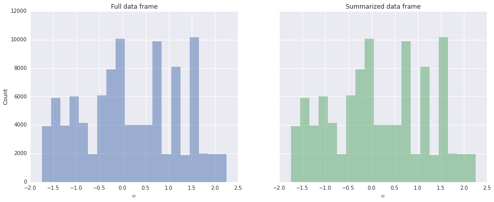
We see that the histograms for \(w\) produced from the full and summarized data frames are identical.
Quantiles
Calculating the mean and variance of our summarized data frames was not too difficult. Calculating quantiles from this data frame is slightly more involved, though still not terribly hard.
Our implementation will rely on sorting the data frame. Though this implementation is not optimal from a computation complexity point of view, it is in keeping with the spirit of pandas’ implementation of quantiles. I have given some thought on how to implement linear time selection on the summarized data frame, but have not yet worked out the details.
Before writing a function to calculate quantiles of a data frame with several columns, we will walk through the simpler case of computing the quartiles of a single series.
u = summ_df.uu.head()0 0
1 48
2 35
3 19
4 40
Name: u, dtype: int64First we argsort the series.
sorted_ilocs = u.argsort()We see that u.iloc[sorted_ilocs] will now be in ascending order.
sorted_u = u.iloc[sorted_ilocs](sorted_u[:-1] <= sorted_u[1:]).all()TrueMore importantly, counts.iloc[sorted_ilocs] will have the count of the smallest element of u first, the count of the second smallest element second, etc.
sorted_n = n.iloc[sorted_ilocs]
sorted_cumsum = sorted_n.cumsum()
cdf = (sorted_cumsum / n.sum()).values
Now, the \(i\)-th location of sorted_cumsum will contain the number of elements of u less than or equal to the \(i\)-th smallest element, and therefore cdf is the empirical cumulative distribution function of u. The following plot shows that this interpretation is correct.
fig, ax = plt.subplots(figsize=(8, 6))

blue, _, red = sns.color_palette()[:3]
ax.plot(sorted_u, cdf, c=blue, label='Empirical CDF');
plot_u = np.arange(100)
ax.plot(plot_u, sp.stats.randint.cdf(plot_u, u_min, u_max), '--', c=red, label='Population CDF');

ax.set_xlabel('$u$');

ax.legend(loc=2);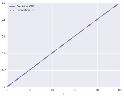
If, for example, we wish to find the median of u, we want to find the first location in cdf which is greater than or equal to 0.5.
median_iloc_in_sorted = (cdf < 0.5).argmin()The index of the median in u is therefore sorted_ilocs.iloc[median_iloc_in_sorted], so the median of u is
u.iloc[sorted_ilocs.iloc[median_iloc_in_sorted]]49df.u.quantile(0.5)49.0We can generalize this method to calculate multiple quantiles simultaneously as follows.
q = np.array([0.25, 0.5, 0.75])u.iloc[sorted_ilocs.iloc[np.less.outer(cdf, q).argmin(axis=0)]]2299 24
9079 49
1211 74
Name: u, dtype: int64df.u.quantile(q)0.25 24
0.50 49
0.75 74
dtype: float64The array np.less.outer(cdf, q).argmin(axis=0) contains three columns, each of which contains the result of comparing cdf to an element of q. The following function generalizes this approach from series to data frames.
def quantile(df, count, q=0.5):
    q = np.ravel(q)

    sorted_ilocs = df.apply(pd.Series.argsort)
    sorted_counts = sorted_ilocs.apply(lambda s: count.iloc[s].values)
    cdf = sorted_counts.cumsum() / sorted_counts.sum()

    q_ilocs_in_sorted_ilocs = pd.DataFrame(np.less.outer(cdf.values, q).argmin(axis=0).T,
                                           columns=df.columns)
    q_ilocs = sorted_ilocs.apply(lambda s: s[q_ilocs_in_sorted_ilocs[s.name]].reset_index(drop=True))

    q_df = df.apply(lambda s: s.iloc[q_ilocs[s.name]].reset_index(drop=True))
    q_df.index = q

    return q_df
quantile(summ_df, n, q=q)| u | v | w | |
|---|---|---|---|
| 0.25 | 24 | 0 | -0.688514 |
| 0.50 | 49 | 1 | 0.040036 |
| 0.75 | 74 | 1 | 1.074817 |
df.quantile(q=q)| u | v | w | |
|---|---|---|---|
| 0.25 | 24 | 0 | -0.688514 |
| 0.50 | 49 | 1 | 0.040036 |
| 0.75 | 74 | 1 | 1.074817 |
np.allclose(quantile(summ_df, n, q=q), df.quantile(q=q))TrueBootstrapping
Another important operation is bootstrapping. We will see two ways to perfom bootstrapping on the summary data set.
n_boot = 10000Key to both approaches to the bootstrap is knowing the proprotion of the data set that each distinct combination of features comprised.
weights = n / n.sum()The two approaches differ in what type of data frame they produce. The first we will discuss produces a non-summarized data frame with non-unique rows, while the second produces a summarized data frame. Each fo these approaches to bootstrapping is useful in different situations.
Non-summarized bootstrap
To produce a non-summarized data frame, we generate a list of locations in feature_df based on weights using numpy.random.choice.
boot_ixs = np.random.choice(summ_df.shape[0], size=n_boot, replace=True,
                            p=weights)
boot_df = summ_df.iloc[boot_ixs]boot_df.head()| u | v | w | |
|---|---|---|---|
| 1171 | 47 | 1 | -1.392235 |
| 9681 | 3 | 1 | 0.018521 |
| 6664 | 13 | 1 | 1.941207 |
| 8343 | 13 | 0 | 0.655181 |
| 3595 | 95 | 1 | 0.972592 |
We can verify that our bootstrapped data frame has (approximately) the same distribution as the original data frame using Q-Q plots.
ps = np.linspace(0, 1, 100)boot_qs = boot_df[['u', 'w']].quantile(q=ps)qs = df[['u', 'w']].quantile(q=ps)fig, ax = plt.subplots(figsize=(8, 6))
blue = sns.color_palette()[0]
ax.plot((u_min, u_max), (u_min, u_max), '--', c='k', lw=0.75,
label='Perfect agreement');
ax.scatter(qs.u, boot_qs.u, c=blue, alpha=0.5);
ax.set_xlim(u_min, u_max);
ax.set_xlabel('Original quantiles');
ax.set_ylim(u_min, u_max);
ax.set_ylabel('Resampled quantiles');
ax.set_title('Q-Q plot for $u$');
ax.legend(loc=2);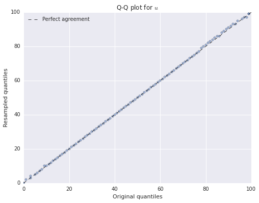
fig, ax = plt.subplots(figsize=(8, 6))

blue = sns.color_palette()[0]
ax.plot((w_min, w_max), (w_min, w_max), '--', c='k', lw=0.75,
        label='Perfect agreement');
ax.scatter(qs.w, boot_qs.w, c=blue, alpha=0.5);


ax.set_xlim(w_min, w_max);
ax.set_xlabel('Original quantiles');

ax.set_ylim(w_min, w_max);
ax.set_ylabel('Resampled quantiles');

ax.set_title('Q-Q plot for $w$');
ax.legend(loc=2);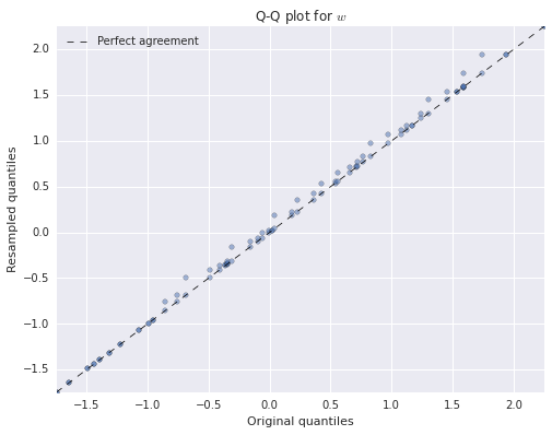
We see that both of the resampled distributions agree quite closely with the original distributions. We have only produced Q-Q plots for \(u\) and \(w\) because \(v\) is binary-valued.
While at first non-summarized boostrap resampling may appear to counteract the benefits of summarizing the original data frame, it can be quite useful when training and evaluating online learning algorithms, where iterating through the locations of the bootstrapped data in the original summarized data frame is efficient.
Summarized bootstrap
To produce a summarized data frame, the counts of the resampled data frame are sampled from a multinomial distribution with event probabilities given by weights.
boot_counts = pd.Series(np.random.multinomial(n_boot, weights), name='count')Again, we compare the distribution of our bootstrapped data frame to that of the original with Q-Q plots. Here our summarized quantile function is quite useful.
boot_count_qs = quantile(summ_df, boot_counts, q=ps)fig, ax = plt.subplots(figsize=(8, 6))
ax.plot((u_min, u_max), (u_min, u_max), '--', c='k', lw=0.75,
label='Perfect agreement');
ax.scatter(qs.u, boot_count_qs.u, c=blue, alpha=0.5);
ax.set_xlim(u_min, u_max);
ax.set_xlabel('Original quantiles');
ax.set_ylim(u_min, u_max);
ax.set_ylabel('Resampled quantiles');
ax.set_title('Q-Q plot for $u$');
ax.legend(loc=2);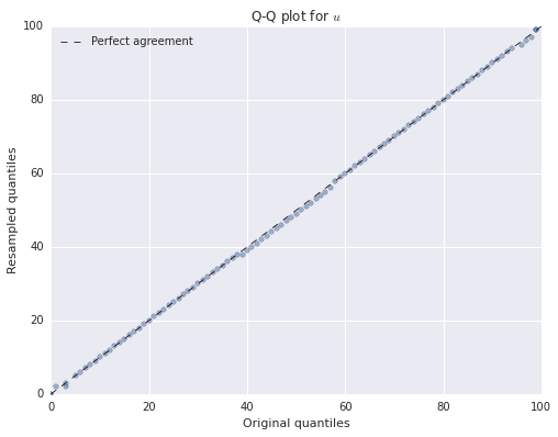
fig, ax = plt.subplots(figsize=(8, 6))

ax.plot((w_min, w_max), (w_min, w_max), '--', c='k', lw=0.75,
        label='Perfect agreement');
ax.scatter(qs.w, boot_count_qs.w, c=blue, alpha=0.5);

ax.set_xlim(w_min, w_max);
ax.set_xlabel('Original quantiles');

ax.set_ylim(w_min, w_max);
ax.set_ylabel('Resampled quantiles');

ax.set_title('Q-Q plot for $w$');
ax.legend(loc=2);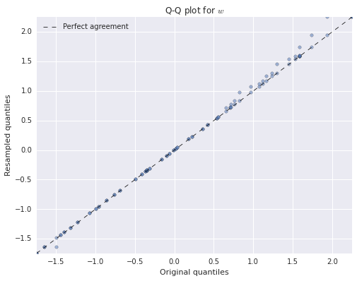
Again, we see that both of the resampled distributions agree quite closely with the original distributions.
Linear Regression
Linear regression is among the most frequently used types of statistical inference, and it plays nicely with summarized data. Typically, we have a response variable \(y\) that we wish to model as a linear combination of \(u\), \(v\), and \(w\) as
\[ \begin{align*} y_i = \beta_0 + \beta_1 u_i + \beta_2 v_i + \beta_3 w_i + \varepsilon, \end{align*} \]
where \(\varepsilon \sim N(0, \sigma^2)\) is noise. We generate such a data set below (with \(\sigma = 0.1\)).
beta = np.array([-3., 0.1, -4., 2.])noise_std = 0.1X = dmatrix('u + v + w', data=df)y = pd.Series(np.dot(X, beta), name='y') + sp.stats.norm.rvs(scale=noise_std, size=N)y.head()0 7.862559
1 3.830585
2 -0.388246
3 1.047091
4 0.992082
Name: y, dtype: float64Each element of the series y corresponds to one row in the uncompressed data frame df. The OLS class from statsmodels comes quite close to recovering the true regression coefficients.
full_ols = sm.OLS(y, X).fit()full_ols.paramsconst -2.999658
x1 0.099986
x2 -3.998997
x3 2.000317
dtype: float64To show how we can perform linear regression on the summarized data frame, we recall the the ordinary least squares estimator minimizes the residual sum of squares. The residual sum of squares is given by
\[ \begin{align*} RSS & = \sum_{i = 1}^n \left(y_i - \mathbf{x}_i \mathbf{\beta}^{\intercal}\right)^2. \end{align*} \]
Here \(\mathbf{x}_i = [1\ u_i\ v_i\ w_i]\) is the \(i\)-th row of the original data frame (with a constant added for the intercept) and \(\mathbf{\beta} = [\beta_0\ \beta_1\ \beta_2\ \beta_3]\) is the row vector of regression coefficients. It would be tempting to rewrite \(RSS\) by grouping the terms based on the row their features map to in the compressed data frame, but this approach would lead to incorrect results. Due to the stochastic noise term \(\varepsilon_i\), identical values of \(u\), \(v\), and \(w\) can (and will almost certainly) map to different values of \(y\). We can see this phenomenon by calculating the range of \(y\) grouped on \(u\), \(v\), and \(w\).
reg_df = pd.concat((y, df), axis=1)reg_df.groupby(('u', 'v', 'w')).y.apply(np.ptp).describe()count 9997.000000
mean 0.297891
std 0.091815
min 0.000000
25% 0.237491
50% 0.296838
75% 0.358015
max 0.703418
Name: y, dtype: float64If \(y\) were uniquely determined by \(u\), \(v\), and \(w\), we would expect the mean and quartiles of these ranges to be zero, which they are not. Fortunately, we can account for is difficulty with a bit of care.
Let \(S_j = \{i\ |\ \mathbf{x}_i = \mathbf{z}_j\}\), the set of row indices in the original data frame that correspond to the \(j\)-th row in the summary data frame. Define \(\bar{y}_{(j)} = \frac{1}{n_j} \sum_{i \in S_j} y_i\), which is the mean of the response variables that correspond to \(\mathbf{z}_j\). Intuitively, since \(\varepsilon_i\) has mean zero, \(\bar{y}_{(j)}\) is our best unbiased estimate of \(\mathbf{z}_j \mathbf{\beta}^{\intercal}\). We will now show that regressing \(\sqrt{n_j} \bar{y}_{(j)}\) on \(\sqrt{n_j} \mathbf{z}_j\) gives the same results as the full regression. We use the standard trick of adding and subtracting the mean and get
\[ \begin{align*} RSS & = \sum_{j = 1}^m \sum_{i \in S_j} \left(y_i - \mathbf{z}_j \mathbf{\beta}^{\intercal}\right)^2 \\ & = \sum_{j = 1}^m \sum_{i \in S_j} \left(\left(y_i - \bar{y}_{(j)}\right) + \left(\bar{y}_{(j)} - \mathbf{z}_j \mathbf{\beta}^{\intercal}\right)\right)^2 \\ & = \sum_{j = 1}^m \sum_{i \in S_j} \left(\left(y_i - \bar{y}_{(j)}\right)^2 + 2 \left(y_i - \bar{y}_{(j)}\right) \left(\bar{y}_{(j)} - \mathbf{z}_j \mathbf{\beta}^{\intercal}\right) + \left(\bar{y}_{(j)} - \mathbf{z}_j \mathbf{\beta}^{\intercal}\right)^2\right). \end{align*} \]
As is usual in these situations, the cross term vanishes, since
\[ \begin{align*} \sum_{i \in S_j} \left(y_i - \bar{y}_{(j)}\right) \left(\bar{y}_{(j)} - \mathbf{z}_j \mathbf{\beta}^{\intercal}\right) & = \sum_{i \in S_j} \left(y_i \bar{y}_{(j)} - y_i \mathbf{z}_j \mathbf{\beta}^{\intercal} - \bar{y}_{(j)}^2 + \bar{y}_{(j)} \mathbf{z}_j \mathbf{\beta}^{\intercal}\right) \\ & = \bar{y}_{(j)} \sum_{i \in S_j} y_i - \mathbf{z}_j \mathbf{\beta}^{\intercal} \sum_{i \in S_j} y_i - n_j \bar{y}_{(j)}^2 + n_j \bar{y}_{(j)} \mathbf{z}_j \mathbf{\beta}^{\intercal} \\ & = n_j \bar{y}_{(j)}^2 - n_j \bar{y}_{(j)} \mathbf{z}_j \mathbf{\beta}^{\intercal} - n_j \bar{y}_{(j)}^2 + n_j \bar{y}_{(j)} \mathbf{z}_j \mathbf{\beta}^{\intercal} \\ & = 0. \end{align*} \]
Therefore we may decompose the residual sum of squares as
\[ \begin{align*} RSS & = \sum_{j = 1}^m \sum_{i \in S_j} \left(y_i - \bar{y}_{(j)}\right)^2 + \sum_{j = 1}^m \sum_{i \in S_j} \left(\bar{y}_{(j)} - \mathbf{z}_j \mathbf{\beta}^{\intercal}\right)^2 \\ & = \sum_{j = 1}^m \sum_{i \in S_j} \left(y_i - \bar{y}_{(j)}\right)^2 + \sum_{j = 1}^m n_j \left(\bar{y}_{(j)} - \mathbf{z}_j \mathbf{\beta}^{\intercal}\right)^2. \end{align*} \]
The important property of this decomposition is that the first sum does not depend on \(\mathbf{\beta}\), so minimizing \(RSS\) with respect to \(\mathbf{\beta}\) is equivalent to minimizing the second sum. We see that this second sum can be written as
\[ \begin{align*} \sum_{j = 1}^m n_j \left(\bar{y}_{(j)} - \mathbf{z}_j \mathbf{\beta}^{\intercal}\right)^2 & = \sum_{j = 1}^m \left(\sqrt{n_j} \bar{y}_{(j)} - \sqrt{n_j} \mathbf{z}_j \mathbf{\beta}^{\intercal}\right)^2 \end{align*}, \]
which is exactly the residual sum of squares for regressing \(\sqrt{n_j} \bar{y}_{(j)}\) on \(\sqrt{n_j} \mathbf{z}_j\).
summ_reg_df = reg_df.groupby(('u', 'v', 'w')).y.mean().reset_index().iloc[shuffled_ixs].reset_index(drop=True).copy()
summ_reg_df['n'] = nsumm_reg_df.head()| u | v | w | y | n | |
|---|---|---|---|---|---|
| 0 | 0 | 0 | 0.425597 | -2.173984 | 14 |
| 1 | 48 | 1 | -0.993981 | -4.174895 | 7 |
| 2 | 35 | 0 | 0.358156 | 1.252848 | 9 |
| 3 | 19 | 1 | -0.760298 | -6.612355 | 17 |
| 4 | 40 | 1 | -0.688514 | -4.379063 | 13 |
The design matrices for this summarized model are easy to construct using patsy.
y_summ, X_summ = dmatrices("""
                           I(np.sqrt(n) * y) ~
                           np.sqrt(n) + I(np.sqrt(n) * u) + I(np.sqrt(n) * v) + I(np.sqrt(n) * w) - 1
                           """,
                           data=summ_reg_df)
Note that we must remove patsy’s constant column for the intercept and replace it with np.sqrt(n).
summ_ols = sm.OLS(y_summ, X_summ).fit()summ_ols.paramsarray([-2.99965783, 0.09998571, -3.99899718, 2.00031673])We see that the summarized regression produces the same parameter estimates as the full regression.
np.allclose(full_ols.params, summ_ols.params)TrueLogistic Regression
As a final example of adapting common methods to summarized data frames, we will show how to fit a logistic regression model on a summarized data set by maximum likelihood.
We will use the model
\[P(s = 1\ |\ w) = \frac{1}{1 + \exp(-\mathbf{x} \gamma^{\intercal})}\].
As above, \(\mathbf{x}_i = [1\ u_i\ v_i\ w_i]\). The true value of \(\gamma\) is
gamma = np.array([1., 0.01, -1., -2.])We now generate samples from this model.
X = dmatrix('u + v + w', data=df)p = pd.Series(sp.special.expit(np.dot(X, gamma)), name='p')
s = pd.Series(sp.stats.bernoulli.rvs(p), name='s')logit_df = pd.concat((s, p, df), axis=1)logit_df.head()| s | p | u | v | w | |
|---|---|---|---|---|---|
| 0 | 1 | 0.709963 | 97 | 0 | 0.537397 |
| 1 | 0 | 0.092560 | 79 | 1 | 1.536383 |
| 2 | 0 | 0.153211 | 44 | 1 | 1.074817 |
| 3 | 1 | 0.923609 | 51 | 0 | -0.491210 |
| 4 | 0 | 0.062077 | 47 | 1 | 1.592646 |
We first fit the logistic regression model to the full data frame.
full_logit = sm.Logit(s, X).fit()Optimization terminated successfully.
Current function value: 0.414221
Iterations 7full_logit.paramsconst 0.965283
x1 0.009944
x2 -0.966797
x3 -1.990506
dtype: float64We see that the estimates are quite close to the true parameters.
The technique used to adapt maximum likelihood estimation of logistic regression to the summarized data frame is quite elegant. The likelihood for the full data set is given by the fact that (given \(u\), \(v\), and \(w\)) \(s\) is Bernoulli distributed with
\[s_i\ |\ \mathbf{x}_i \sim \operatorname{Ber}\left(\frac{1}{1 + \exp(-\mathbf{x}_i \gamma^{\intercal})}\right).\]
To derive the likelihood for the summarized data set, we count the number of successes (where \(s = 1\)) for each unique combination of features \(\mathbf{z}_j\), and denote this quantity \(k_j\).
summ_logit_df = logit_df.groupby(('u', 'v', 'w')).s.sum().reset_index().iloc[shuffled_ixs].reset_index(drop=True).copy()
summ_logit_df = summ_logit_df.rename(columns={'s': 'k'})
summ_logit_df['n'] = nsumm_logit_df.head()| u | v | w | k | n | |
|---|---|---|---|---|---|
| 0 | 0 | 0 | 0.425597 | 5 | 14 |
| 1 | 48 | 1 | -0.993981 | 7 | 7 |
| 2 | 35 | 0 | 0.358156 | 8 | 9 |
| 3 | 19 | 1 | -0.760298 | 12 | 17 |
| 4 | 40 | 1 | -0.688514 | 9 | 13 |
Now, instead of each row representing a single Bernoulli trial (as in the full data frame), each row represents \(n_j\) trials, so we have that \(k_j\) is (conditionally) Binomially distributed with
\[k_j\ |\ \mathbf{z}_j \sim \operatorname{Bin}\left(n_j, \frac{1}{1 + \exp(-\mathbf{z}_j \gamma^{\intercal})}\right).\]
summ_logit_X = dmatrix('u + v + w', data=summ_logit_df)As I have shown in a previous post, we can use statsmodels’ GenericLikelihoodModel class to fit custom probability models by maximum likelihood. The model is implemented as follows.
class SummaryLogit(GenericLikelihoodModel):
    def __init__(self, endog, exog, n, **qwargs):
        """
        endog is the number of successes
        exog are the features
        n are the number of trials
        """
        self.n = n

        super(SummaryLogit, self).__init__(endog, exog, **qwargs)

    def nloglikeobs(self, gamma):
        """
        gamma is the vector of regression coefficients

        returns the negative log likelihood of each of the observations for
        the coefficients in gamma
        """
        p = sp.special.expit(np.dot(self.exog, gamma))

        return -sp.stats.binom.logpmf(self.endog, self.n, p)

    def fit(self, start_params=None, maxiter=10000, maxfun=5000, **qwargs):
        # wraps the GenericLikelihoodModel's fit method to set default start parameters
        if start_params is None:
            start_params = np.zeros(self.exog.shape[1])

        return super(SummaryLogit, self).fit(start_params=start_params,
                                             maxiter=maxiter, maxfun=maxfun, **qwargs)
summ_logit = SummaryLogit(summ_logit_df.k, summ_logit_X, summ_logit_df.n).fit()Optimization terminated successfully.
Current function value: 1.317583
Iterations: 357
Function evaluations: 599Again, we get reasonable estimates of the regression coefficients, which are close to those obtained from the full data set.
summ_logit.paramsarray([ 0.96527992, 0.00994322, -0.96680904, -1.99051485])np.allclose(summ_logit.params, full_logit.params, rtol=10**-4)TrueConclusion
Hopefully this introduction to the technique of summarizing data sets has proved useful and will allow you to explore medium data more easily in the future. We have only scratched the surface on the types of statistical techniques that can be adapted to work on summarized data sets, but with a bit of ingenuity, many of the ideas in this post can apply to other models.